
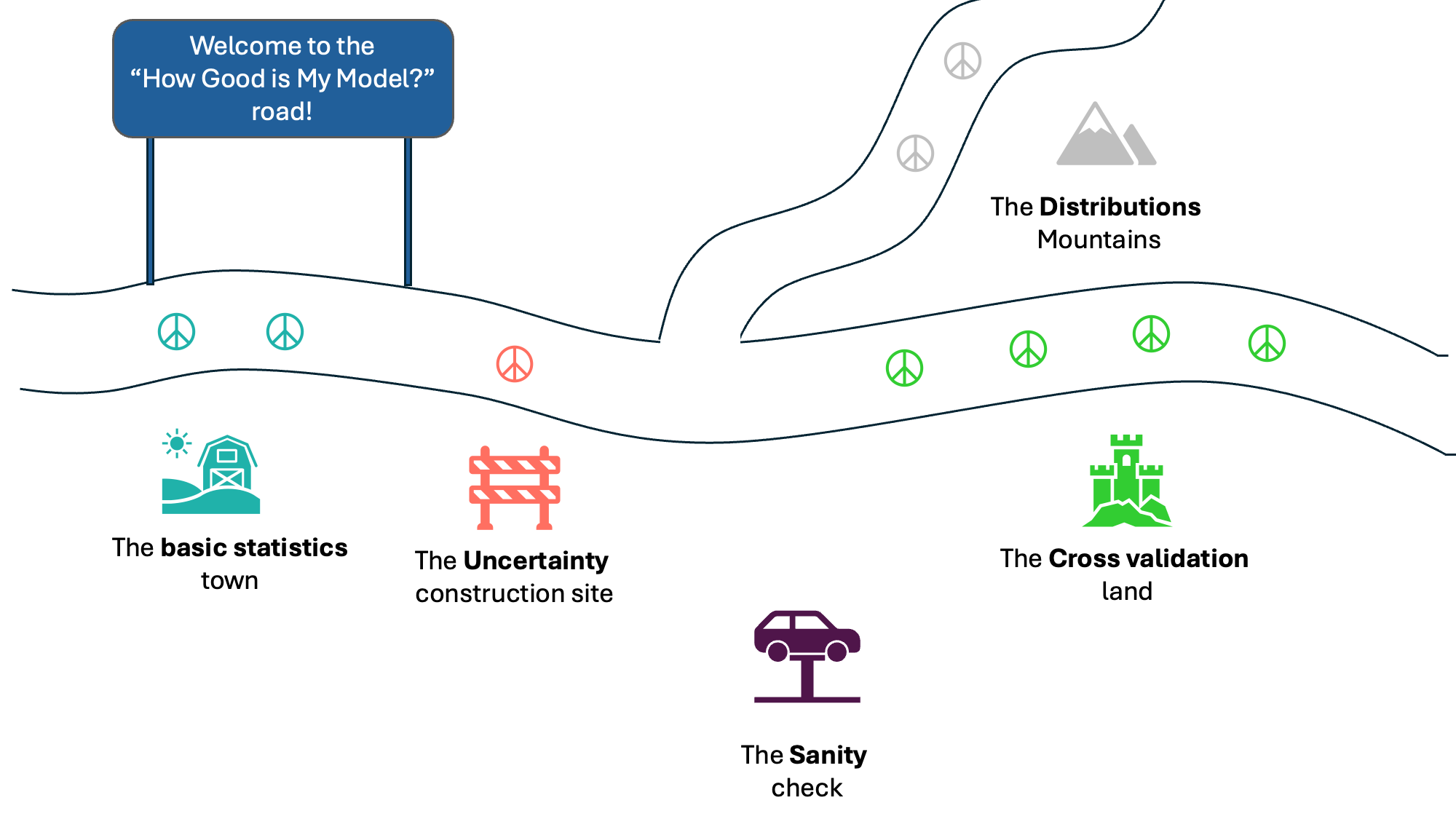
How Good is My Model? Part 4: To Compare, or Not to Compare
Published:
In this post, I go back to the “How Good is My Model?” lane and continue the journey. However, since the next stop is the “Cross-Validation land,” which in my field is mainly about model comparison, one needs to go through this sanity check before moving to comparison. This check should indicate whether I am ready to start comparing models—or not yet.
Let’s recall the last post in this series, where I used analytical and empirical approaches on a test-set residuals sample to estimate the best- and worst-case scenarios for my model’s true performance.
I did so by saying that the assumption about the model’s residuals is that they follow a normal distribution. Therefore, the only things I needed to construct this distribution are the mean (µ) and standard deviation (σ).
If I know µ and σ, I can construct any normal distribution because these are the only two parameters controlling its behavior.
Now that I have an estimate of how my model would generally perform, one might think it is time to start comparing it to other models. Right?
Not really…
Getting a residual distribution of a test set tells me how off this model was on this test set.
But… it does not tell me whether I should listen to the model or not!
What do I mean by “listen to the model”?
I mean that there are signals that can tell me whether my model was truly learning or whether it was playing games on me.
Just because something “works” doesn’t mean it is “right.”
And if I want to do impactful science, I need to distinguish between what is “working right” and what is “just working.”
This post is about that sanity check:
the things I can do after testing on a test set to ensure that my model truly learned,
and that there is nothing obvious left to learn.
This post is accompanied by a notebook to reproduce the figures and explore the concepts shown below.
TL;DR 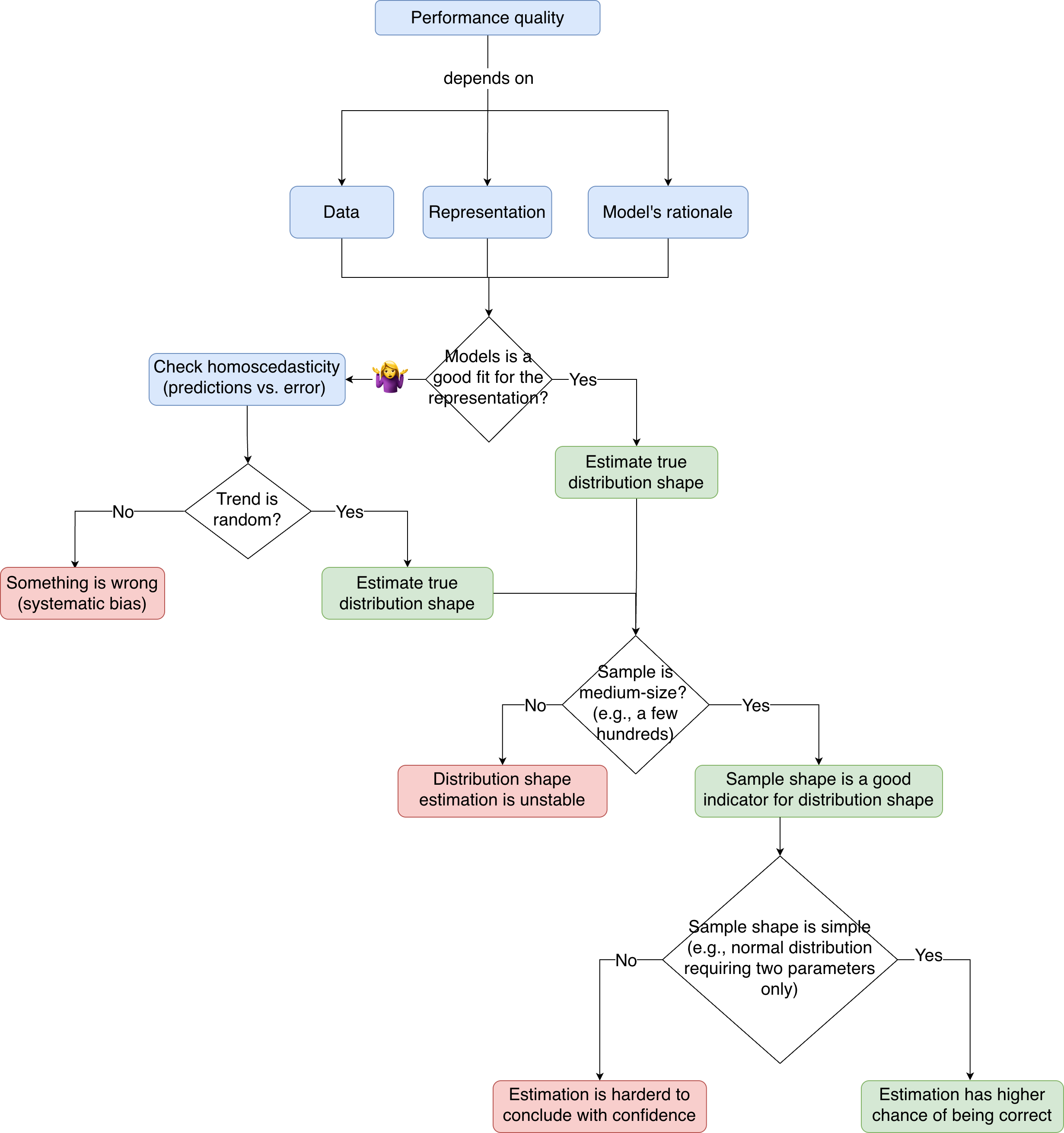
Misunderstanding the normality assumption of model residuals
In that post, and above again, I assumed that a model’s performance follows a normal distribution. But this is not accurate.
Normality of residuals turns out to be an assumption only for linear regression models, and it is important mainly when one wishes to perform significance analysis (perhaps there will be a chance to explore this in depth later).
Outside this very specific scenario, a model’s residual distribution is assumption-free. It can follow any distribution, depending on how the model learned patterns in the data.
And this puts me in a pickle. If the true distribution is not necessarily normal, how can I construct this true distribution from my sample?
Well, a sample—even when small—tells me something about the shape of its distribution.
Figure 1 shows a plot from the last technical post. It shows three different families of distributions and what samples of different sizes look like when randomly drawn from each one. Four things can be learned:
- The spread of a distribution (i.e., width/variance) is easily captured from tiny randomly drawn samples (e.g., only a few tens of examples).
- Samples of a few hundreds are enough to estimate the distribution family (e.g., normal, bimodal, lognormal).
- Samples of several hundreds to thousands are enough to roughly estimate the contour of the distribution.
- For example, the samples in the second row, second column already indicated that the distribution is bimodal, but the density between the two peaks was off and became sharper only at
n = 500andn = 1000.
- For example, the samples in the second row, second column already indicated that the distribution is bimodal, but the density between the two peaks was off and became sharper only at
- Estimating the exact shape—including tail and skew behavior—is much harder and requires a much larger number of examples.
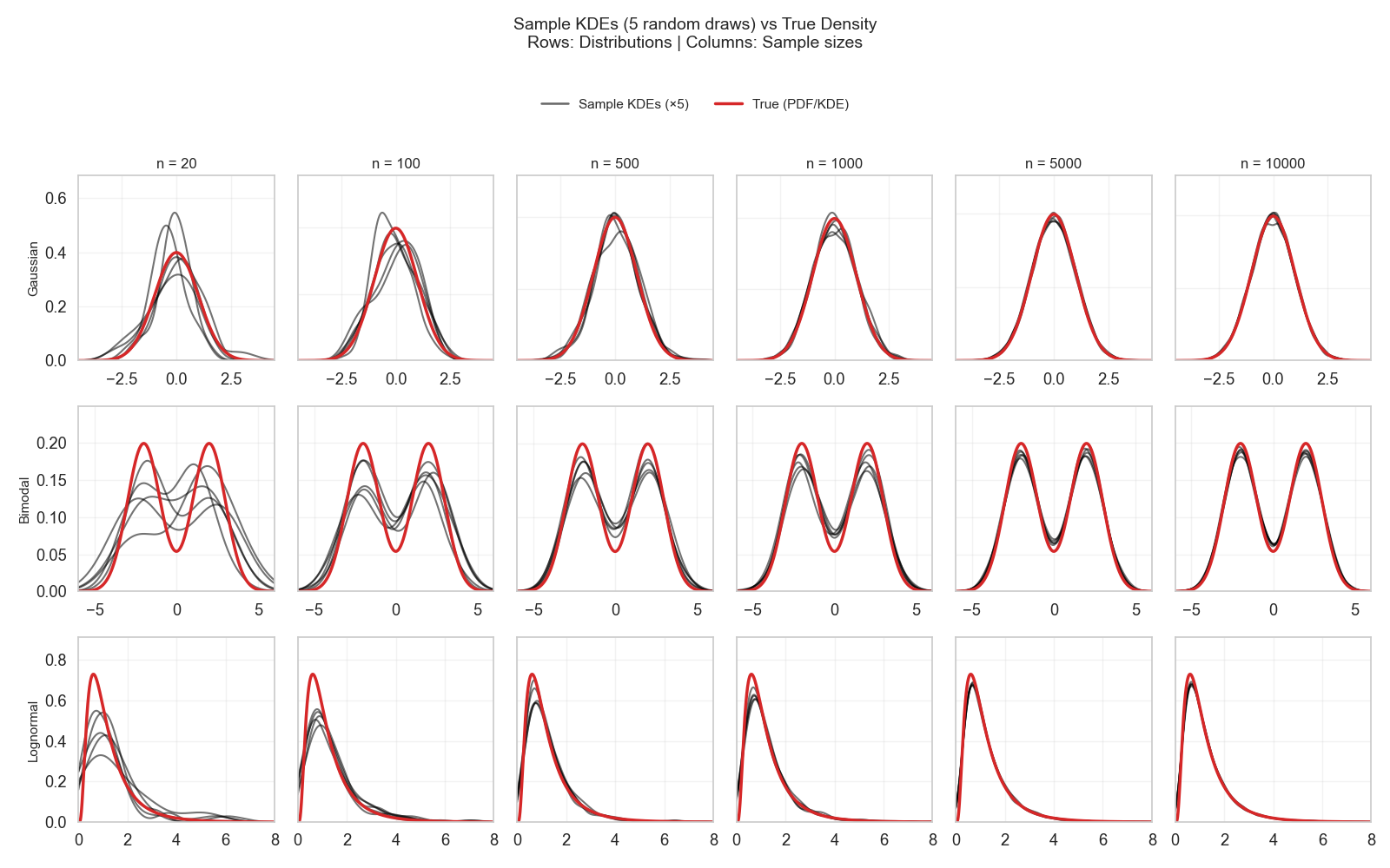
So, the takeaway is that even when one does not know the original distribution, if a sample is of medium size and drawn randomly, one can estimate the family and rough contour of the distribution.
Knowing that my test set had 353 molecules (i.e., examples), I have a good chance that the shape my sample shows will at least indicate the family of its distribution.
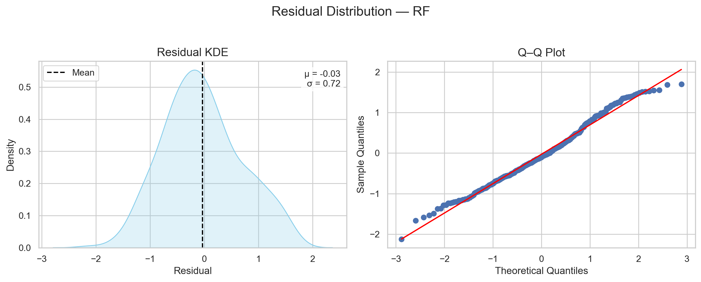
As shown in Figure 2, the shape shows a single peak and symmetry around the peak. This is a sign of normality.
Of course, I am not blind to the lump on the right side of the distribution. But this can be explained in two ways:
- Expected sampling variability (check the sample shapes in Figure 1, first row).
- Systematic bias in my setup (this is what I will try to explore in this post).
Either way, the initial assumption of normality seems to have a decent chance of holding (in this specific case).
So, while the conclusions from the last post turned out to be correct—by chance—it remains vital to know that normality is not a general assumption.
Next time I get a residual sample, I need to check its size and shape to get a feeling for the distribution family it originated from.
Then, I will need to know which parameters must be estimated to construct this distribution, and how to estimate them.
In this case, and for normal distributions generally, the parameters to estimate are µ and σ.
But if my sample indicated a bimodal distribution, for example, then I would need to estimate two µ’s and two σ’s (one pair for each mode).
As a rule of thumb, the more parameters to estimate from the same number of examples, the less confidence one has in their estimates.
So, even if a model’s residual distribution is generally assumption-free, having it follow a normal distribution serves me greatly if I wish to speak with confidence.
Before distribution shape
Before jumping into figuring out which distribution my residuals sample came from, I first need to assess the quality of the performance on the test set.
To know if my model’s performance on this test set is trustworthy, I need to make sure I have sorted my ducks correctly 🐥.
And I have three ducks to sort. 🐥🐥🐥
- The training and testing data are i.i.d.
- The representation of the data that is given to a model is faithful.
- The model has the correct rationale to map between the representation and the task it is predicting.
Let me further explain each duck to clarify what it actually means.
Data are i.i.d.
The last post on distributions detailed this part to some extent. I went through examples of aqueous-solubility datasets and inspected whether they fulfill the i.i.d. condition.
One dataset grossly fell short on the “identically distributed” condition, and it was straightforward to identify how a model trained on this dataset would be destined to fail. The problem was ill-defined; therefore, any evaluation of the model would likely be misleading.
The other dataset was a great effort at generating a random, identically distributed sample, but the independence condition was harder to assert and will need its own post later. One can check this post to see a simulation of what happens to performance when a dataset violates independence.
So, the i.i.d. condition is required to ensure that the model is learning the thing I want it to learn.
If these conditions are violated, this becomes a source of error beyond the model’s capabilities.
Representations are faithful
This is discussed a lot, but often without highlighting its importance from the model’s point of view.
The model does not see data; it sees a representation.
The model does not see a molecule or understand what a molecule is; it only sees whatever we represent the molecule as.
Since machine learning (ML) is about distributions and math, a model needs a numerical representation of any input data.
If it is a molecule, text, or image, it must be converted to numbers.
Anything humans process in raw form, the machine can only see as numbers.
The job of turning a raw format into numbers is producing a representation.
This representation must be as faithful to the original raw format as possible to ensure the model sees what I intend it to see.
So, how is this done?
Consider a generic example before tailoring it to molecules in a later post: predicting a person’s height.
Each data point in a sample corresponds to a human being.
How can I convert a human being into numbers that help a model predict height?
One option is to describe each human in quantifiable descriptors.
This is very broad—there can be infinite aspects to quantify!
How old are they? How many siblings do they have? What is their eye color? How many pairs of pants do they own? How many organs do they have? etc.
If I want to predict height, the number of pants is likely irrelevant (unless I have reason to suspect correlation).
Describing someone by the number of organs is also not discriminative because most people have the same number.
Eye color is probably irrelevant, but one might argue it weakly indicates certain genes that could be related to height.
Okay, keep it; it will not hurt. But expectations should be modest.
Etc., etc., etc. (Figure 3)
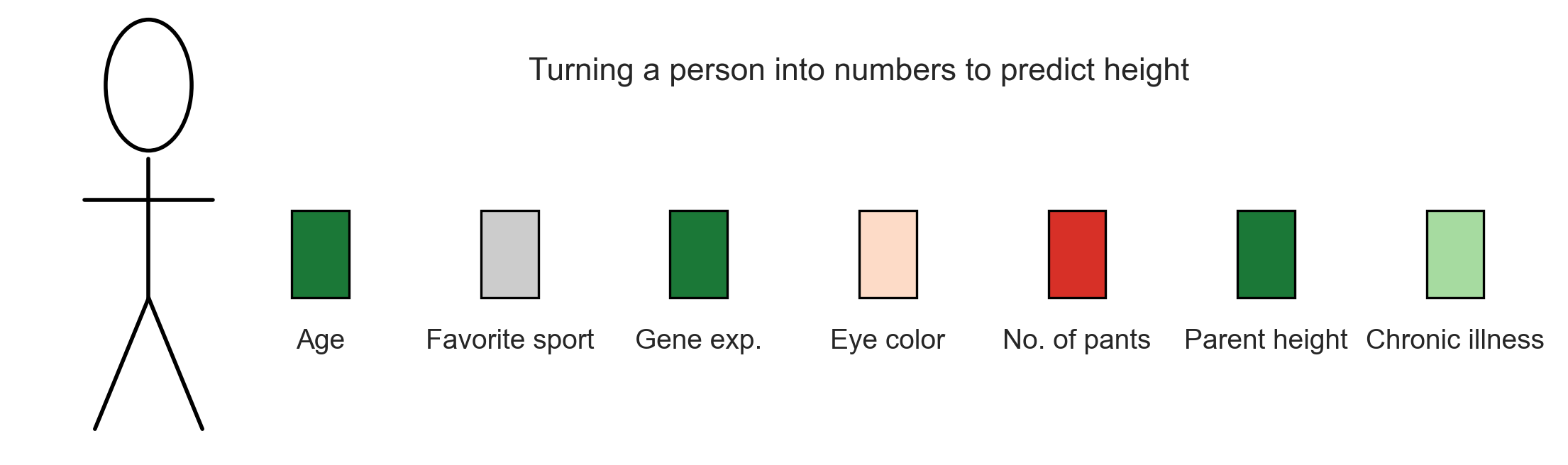
This is how one converts a physical entity that humans process naturally—but cannot easily formalize—into numbers.
And this is what we feed a model. This is what the model sees…
Models do not see what we see. They see what someone thinks we see.
Please let this sentence sink in…
In short, the descriptors I use to describe my data should be relevant to the thing I am trying to predict (as decided by me or by someone I trust to make this representation).
This depends on how much I (or the trustee) know about the problem.
For individual height, much research and accumulated knowledge indicate that factors like genes, geography, and socioeconomic status are key players.
To convert a human being into numbers that help infer height, such factors should enter the representation (also called featurization).
Then my model will not see a human being, but a numeric representation of features believed to be relevant to the target.
Are we aware of every single feature that determines someone’s height?
Probably not.
Because of this, our representation will be incomplete.
Hence, the model will process incomplete information.
This is a source of error beyond the model’s capabilities.
The model’s rationale is solid
A model is a sequence of equations that attempts to capture the relationship between the representation it sees and the task it predicts.
Each model has assumptions about what these representations are and how they should interact to predict an outcome.
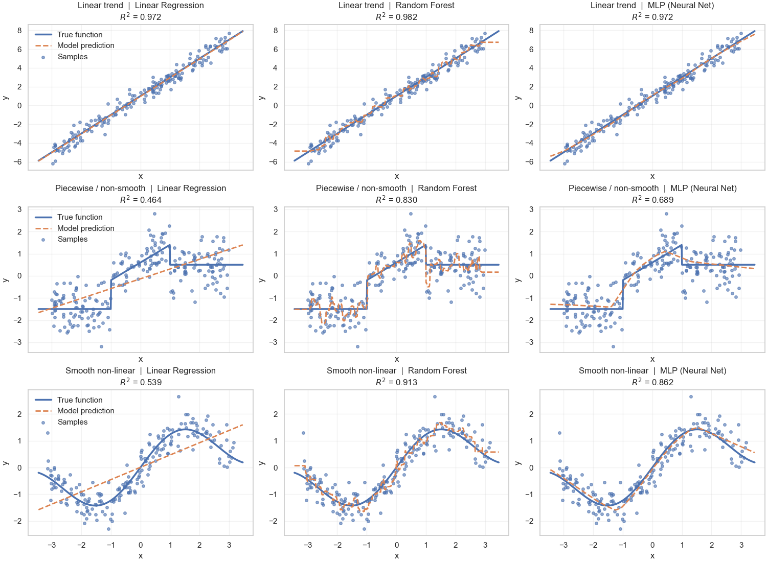
Pairing the representation with the model should be done mindfully; not every model works well with every representation (Figure 4).
Another post (or series) may walk through the worldviews of different model families. Here, a brief list suffices.
The simplest ML model is linear regression (LR). It has a simple worldview.
An LR model assumes each feature in the representation affects the output independently and linearly.
What does this mean?
If we take height with features like gene expression and nationality, LR assumes that each feature has a specific weight in deciding height, and features do not influence each other.
So an LR model can make conclusions like: gene expression explains 30% of the variability in height, while nationality explains 20%.
What LR will never conclude is something like:
- When someone comes from THIS nation and has THIS gene, 35% of the variability is explained.
- When gene expression is between these values, 15% is explained, but between those other values, 25% is explained.
LR does not consider that interacting features can change the outcome,
nor that a single feature can affect the outcome differently in different regions.
A model like random forest (RF) does consider both. It allows features to have different effects across regions and to interact.
However, RFs assume the data are governed by rules, and they try to extract those rules.
But what if the data have trends rather than rules, and these trends are smooth and more abstract than what is present in the data at hand?
Then neural networks (NNs) have assumptions that can capture moving trends rather than strict rules.
So, if someone knows the representation relates nonlinearly to the target but uses LR, the model will produce large errors because it is not suitable for the representation.
If someone knows the representation has fluid trends rather than strict rules, then an RF may also be a mismatch.
Understanding what representations I have and what assumptions a model makes can already indicate whether my setup makes sense.
Putting it all together
So, how does the talk about i.i.d. data, faithful representation, and solid model rationale help me assess the quality of my test residuals?
The assumption is: if someone used good data, a faithful representation, and an appropriate model, then the predictions should be mostly correct.
But because things are never perfect, the model is bound to make errors. These errors arise from suboptimal data curation, missing important features, and imperfect model architecture.
What I want to assert is that a model has learned whatever there is to learn in the setup it is given.
It is no longer—perhaps never has been—about perfect prediction or understanding of “the problem,” but rather, a somewhat perfect prediction/understanding of “whatever I have right now.”
I believe ML tasks—here and elsewhere—can be framed as:
- If I want to understand and predict a problem (e.g., aqueous solubility) → I need enough random i.i.d. data that generously cover the problem space and as faithful a representation as possible.
- If I want to understand and predict whatever data I have right now (e.g., a dataset of a few thousand molecules with apparent solubility at pH 7.4), even if it violates randomness and independence → I need as faithful a representation as possible.
- Note: violating the identically distributed part is not tolerated. Both cases require well-defined, clean, and untampered data.
- If I want to understand and predict either case given a faithful representation → I need to pick the right model.
How to tell if data are random i.i.d.? Check this post.
How to tell if a representation is faithful? I am aware of two ways:
- I know the most expert person in the area and they told me everything known about the problem so far.
- I find a model that—using this representation—learns and generalizes very well.
How to tell if a model is good? A model is not absolutely good or bad. A model is either:
- Not a good fit for the current data and representation.
- As good as the data and representation are.
So, when a model performs disappointingly, the first step is to double-check whether it was the right fit to the best of my knowledge.
- If yes, then I need to go back and work on my representation and data; these will be the bottleneck.
- If no, then another model or architecture may work better with this data and representation.
- If I cannot tell, then I am in the pickle currently present in my field… One can only search for an expert and learn1.
Machines start learning only after we ourselves have learned. They are forever dependent on whatever we give them (data, representation, and rationale).
How to spot the faults in my setup?
Let me recall what happened in this post.
I performed an ML pipeline as follows:
- A dataset of 1,763 molecules with apparent solubility at pH 7.4.
- A list of descriptors available from RDKit: physicochemical (weight, polarity, electronegativity) and structural (branching, complexity).
- An RF model trained on 80% of the data and tested on the remaining 20% (353 molecules).
So, I chose a model and gave it data in a certain representation. This specific setup contains information to be learned, and this is what I want to judge my model against.
Did my model learn whatever is there in this specific setup?
So far, I had been looking at the error-distribution plot of this sample (Figure 2) and assuming it is “good enough” to construct the true performance distribution.
But if I use a different plot—errors against the predictions themselves—I get the scatter in Figure 5. The x-axis shows the prediction for each molecule in the test set, and the y-axis shows the error for each predicted value.
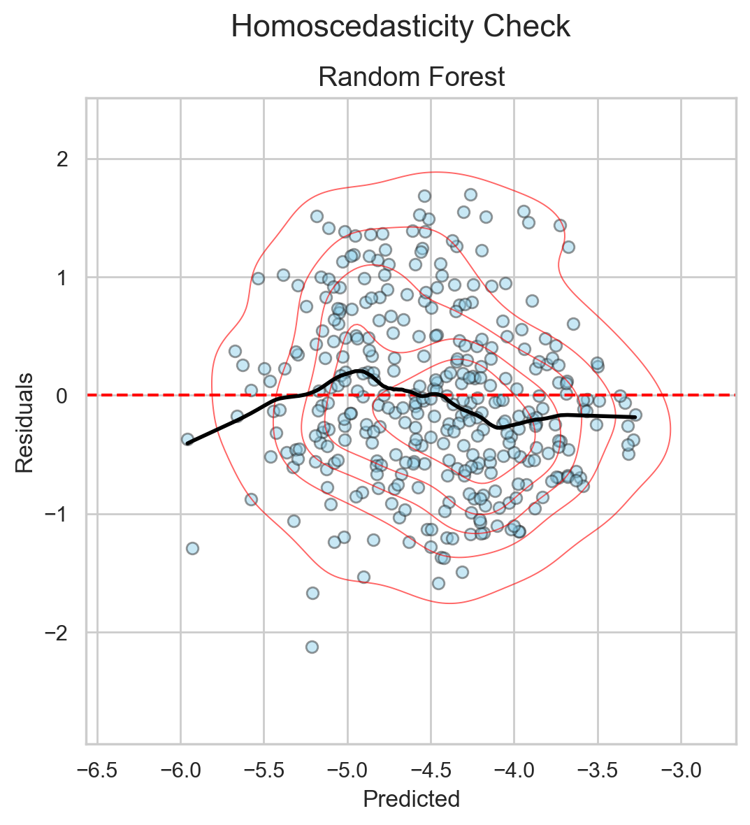
This figure helps me understand how my model errs across prediction ranges.
For example, when the model makes small predictions, are those usually correct (error ≈ 0) or high?
I look for ranges where errors are systematically too big or too small.
If a model learns the structure in the data correctly, this plot will be pretty random with no observable trends (i.e., homoscedastic). Points scatter almost equally above and below the horizontal line at error = 0.
When I see this behavior, I know the model is not biased toward any particular prediction range. This suggests the model has learned whatever information was present.
Since this is the trend I see in Figure 52, I conclude that this setup—this dataset + these RDKit descriptors + the RF model—is a match made in heaven.
If I want more accurate predictions, I need to improve my data or my representation.
But we were quite lucky to have a match from the first shot (well, not really—this aligns with much of the literature and with what we showed in our latest preprint as well).
Let’s see what this plot looks like if the match of dataset, representation, and model is faulty.
I trained the same dataset and representation using a simple linear regression (LR) model and a fluid nonlinear multi-layer perceptron (MLP) model.
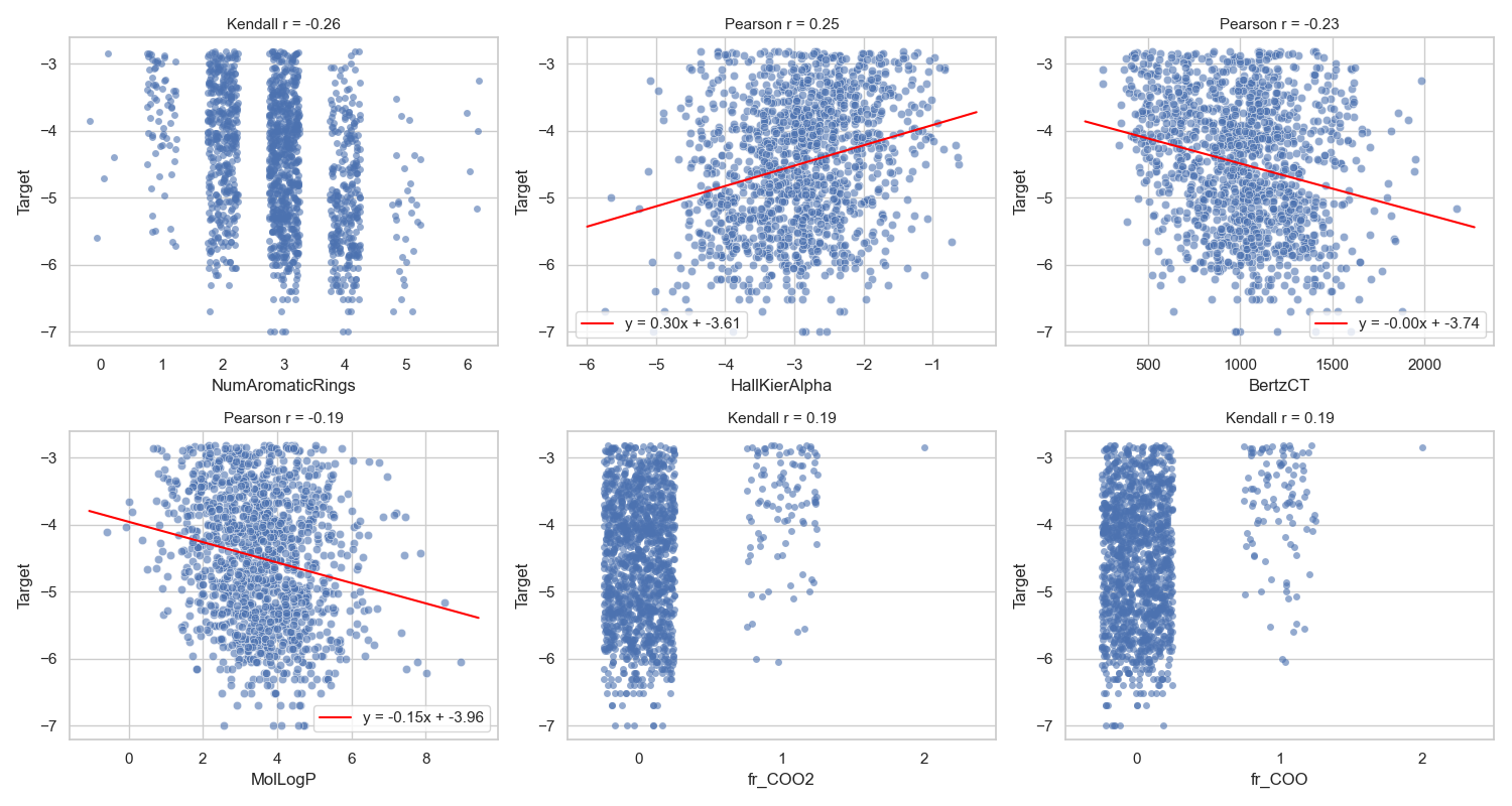
Before running these models, my assumption was that LR would perform badly. In preliminary analysis, the representation did not have strong linear relationships with the target (Figure 6).
Since LR is about linearity, this is already a mismatch.
For the MLP, I suspected performance similar to RF because both handle nonlinearity well.
However, the results led me to uncover something very interesting about my data—something I did not know before putting these diagnostic plots side by side.
I first checked the residual plots of the two models, compared their best- and worst-case performance to the RF model, and then examined the diagnostic plots.
Figure 7 shows that the test-set residuals of the LR and MLP models likely originate from a normal distribution, similar to RF.
This makes it easier to compare the three, since they share a comparable level of confidence in estimating their true distributions.
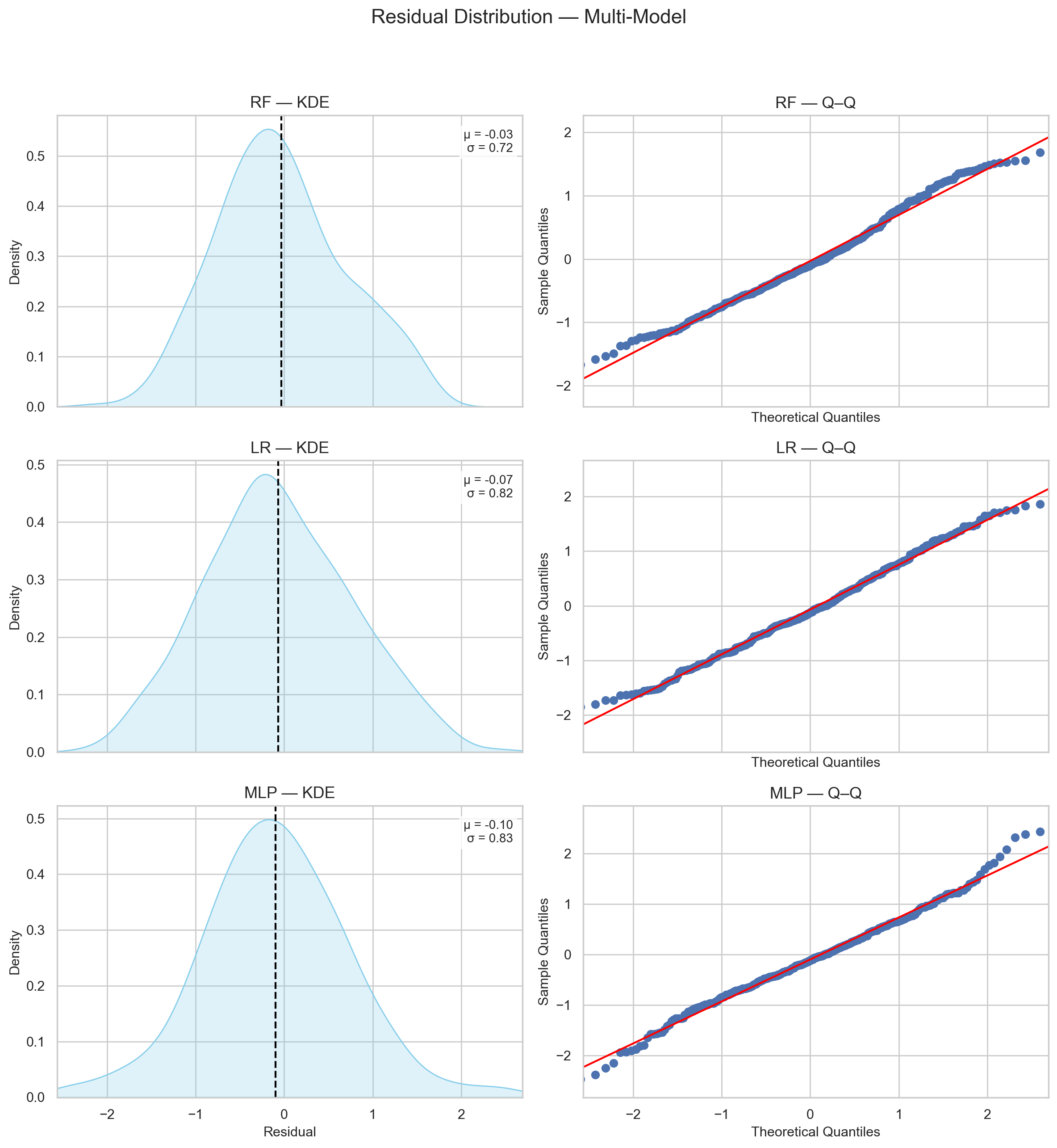
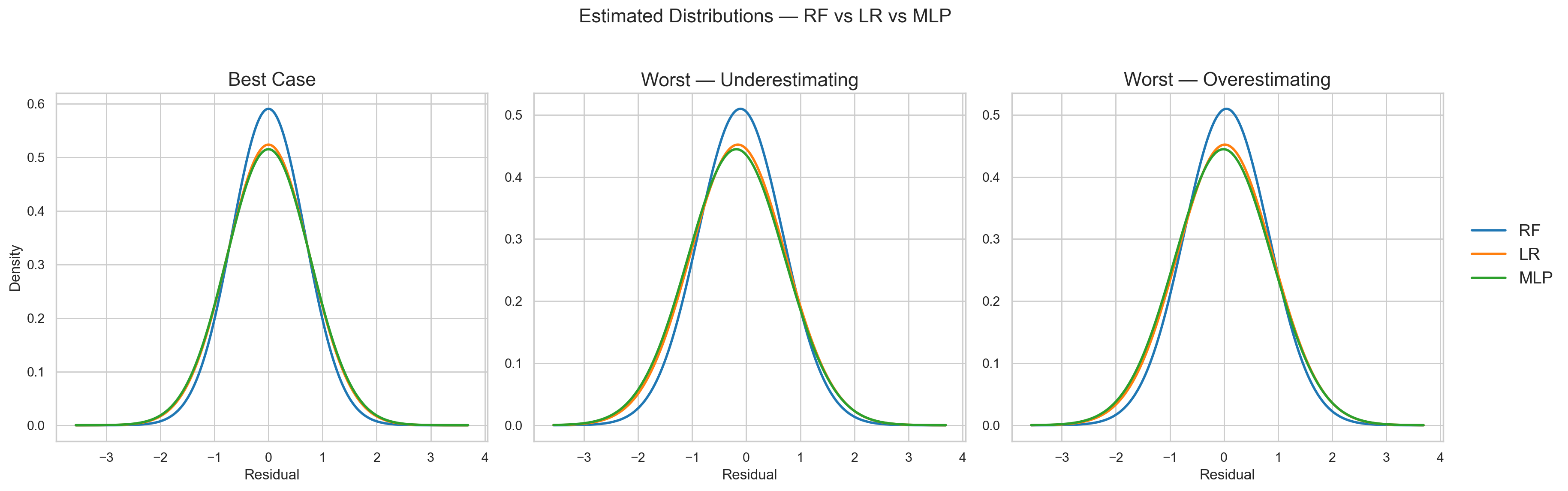
Figure 8 shows the best- and worst-case scenarios for the three models. The LR model shows worse performance than RF because its distribution has larger variance in all cases. This was expected.
However, what I did not expect was that the MLP’s performance is worse than RF and almost the same as LR!
Looking at the diagnostic plot in Figure 9, the LR model shows heteroscedasticity (i.e., errors vary across prediction ranges). This could be explained by the lack of modeled nonlinearity.
However, the heteroscedastic trend also appears for the MLP model—even more strongly.
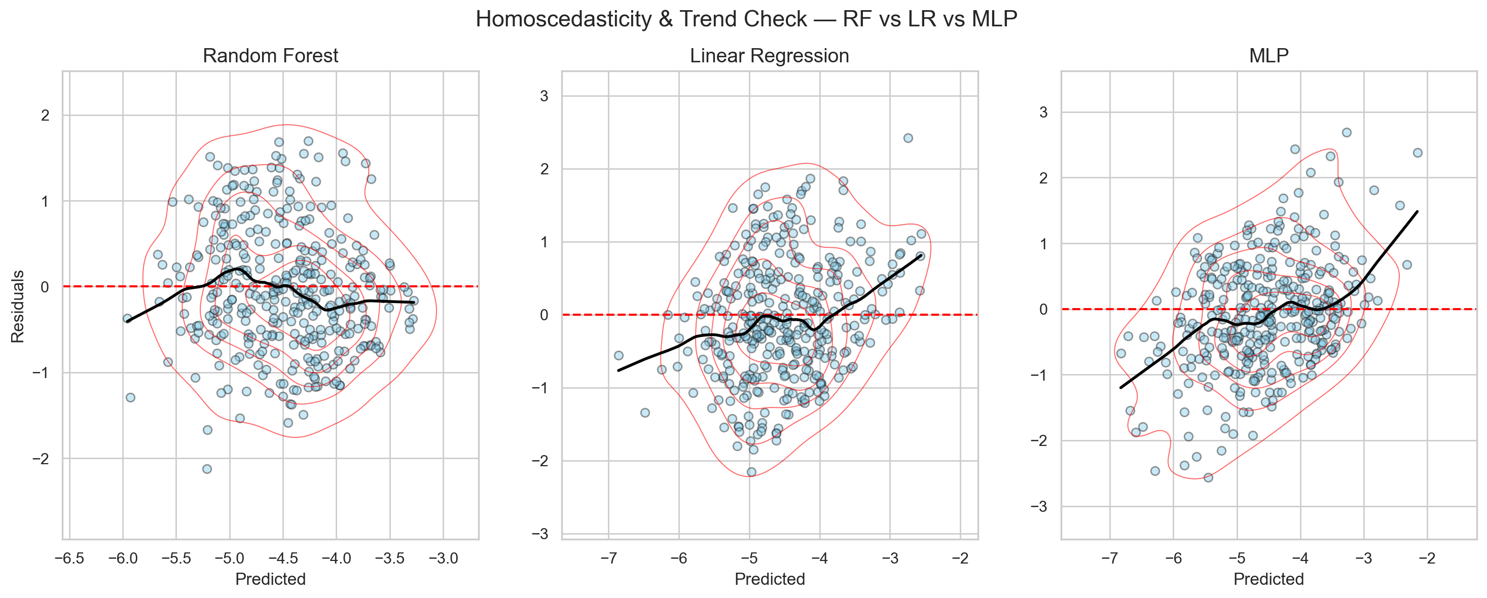
So, what on earth is happening?
What is common between LR and MLP, but different from RF—making RF better suited for my data and representation?
Smooth global function vs. piecewise local function
That is the difference between RF and LR/MLP (refer back to Figure 4).
- For LR, the global function is strictly linear—a single straight line or hyperplane.
- For MLP, the function is fluid and can fit complex patterns, but it remains a smooth function3.
What does this tell me?
It tells me that the relationship between my dataset and the representations is non-smooth. The behavior of my molecules changes abruptly with the features I use, and there is no single smooth function that fits it well.
Therefore, the RF rationale fits best. RF splits the space by feature thresholds and fits local functions rather than a single global function.
What is making my dataset jumpy? And should I expect it to be jumpy?
This is a question for later. The interesting takeaway is precisely this question.
It was not about comparing models to select a “best performer.” It was the simple act of listening to different models, understanding what they are trying to say, and realizing that I needed to go back to my data.
The different models—with their different behaviors, and with a real risk that all of them would fail to generalize to new molecules—still told me where to look next to improve my understanding4!
If that is all these models achieved, I would still call it a success for now.
Let’s recap
- Normality isn’t universal: it mainly matters for linear regression and significance testing. However, it helps a lot when the errors do follow a normal distribution.
- One can infer the distribution shape if they have a medium-size sample
- Assessing a model’s performance starts before comparison — it begins with checking whether the setup itself makes sense.
- The data, representation, and model must be in harmony before their outcomes can be trusted.
- Each model offers a different worldview: linear, piecewise, or smooth and continuous.
- Listening to how they each fail or succeed reveals more about the data than about the models themselves.
- The goal is not to crown a “best performer,” but to learn what the performance means.
- to understand where the signal ends, where the noise begins, and what the model is really trying to say.
Another approach, when one cannot tell and does not want to consult an expert, is to try things blindly (trial and error). This is not my favorite approach, but it is valid. The caveat, in my opinion, is that one needs to be extremely humble with it and never use it to assert confidence or knowledge. At best, it helps one “learn a bit more,” not “solve a problem.” ↩
The trend is more or less homoscedastic. With a somewhat small test set, perfect randomness is not expected. Where randomness is less prominent, it is likely sampling variability to the best of my knowledge. ↩
Hypothetically, a neural network can be guided to detect non-smooth behavior. However, this requires increasing depth and width, which inflates the number of parameters. As mentioned earlier, the more parameters to estimate, the more data are needed to estimate them with confidence. In a data-limited regime like ours, if the global function is non-smooth, it becomes inefficient and uncertain to demand that an NN learn it. ↩
The performance of the three models also says something about my representation. This will be discussed later as well. ↩