To help myself understand what a model is, I will go, as usual, elemental. I will try to see what the simplest possible form of a model is, and build my intuition about it one step at a time.

What is a model?

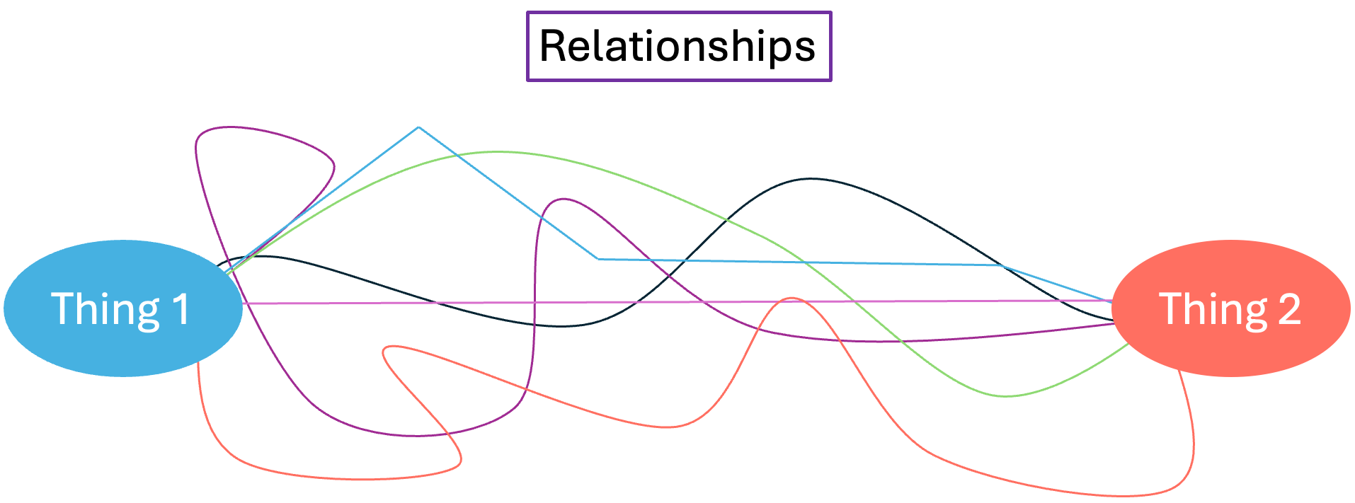
A model is a tool that uncovers (models) a relationship between two things.

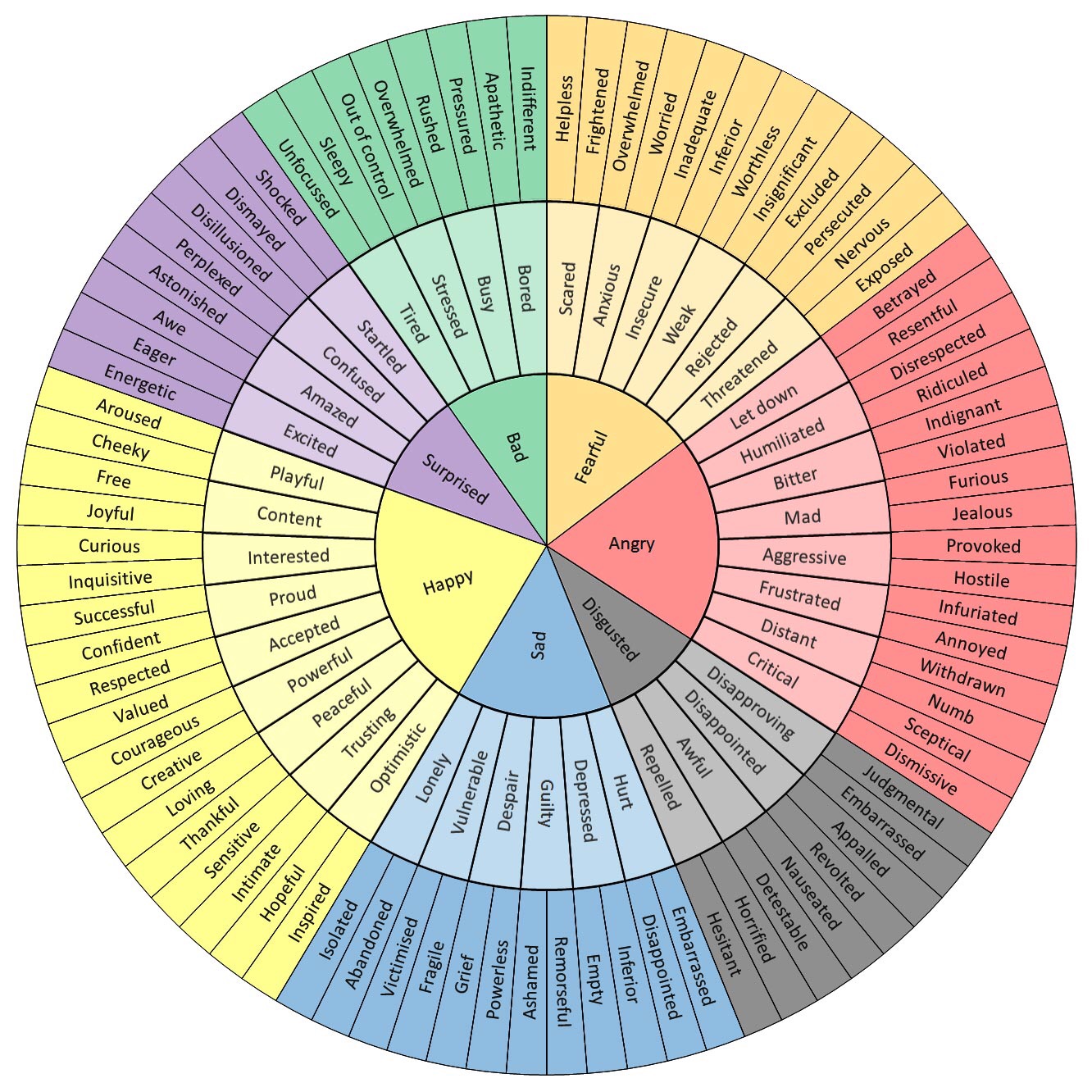
Let us think about feelings and behaviors, for example. I believe we can agree that there is a relationship between them. If someone is angry, they are more likely to be fidgety and make their surroundings reactive. If someone is relaxed, they are more likely to stay in a confined space and move smoothly.

The ability to describe this sequence of angry → reactive, relaxed → smooth, etc., is exactly what a model does. It finds a relationship that maps between something (feelings) and another thing (behavior).

This mapping and this relationship are what any model is trying to express. And this relationship can range from simple to intricate.

Different types of things (variables)

The possible relationships that can exist between two things begin by identifying the type of these two things. In the lingo of machine learning, a thing that can have different outcomes is referred to as a variable¹.

There are two main classes used to describe a variable: qualitative and quantitative. Each of these classes restricts the way one might think about relationships. Therefore, they restrict what a certain model can do about them.

Let us further explain these classes.

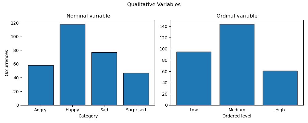
Qualitative variable

Qualitative variables describe an entity outside the numerical realm. They obey simple mathematical operations strictly contained within the realm of discrete mathematics. These qualitative variables split into two categories.

1. Nominal (i.e., orderless descriptors like happy, angry, or cat, dog): These descriptors merely name things. They do not have notions of order, magnitude, or spacing.
2. Ordinal (i.e., ordered descriptors like low, medium, or neutral, good): These descriptors are also merely names, but they have order (i.e., medium is “higher” than low) and spacing (i.e., medium is in the middle of low, medium, and high). However, the spacing is not quantified (i.e., one does not know what the “distance” between low and medium is).

The mathematical operations one can apply to nominal variables will be things like logical operations (e.g., NOT, AND, OR, XOR), set theory (e.g., \(\cup\), \(\cap\), \(\subset\)), graph theory, and discrete probability. Things can happen together, partially, or not happen. They can happen together equally or conditionally. And so on.

With ordinal variables, the same operations apply, but now one can add comparison operations (e.g., \(>, <, \ge\)).

Quantitative variables

The other class of variables is the numerical one. This is where math can do its full magic! But one still needs to be careful about which math does which magic.

The number line stretches from \(-\infty\) to \(+\infty\) with all possible numbers. And math is most powerful when it deals with the full rich spectrum of the number line. However, not all numerical variables span these numbers.

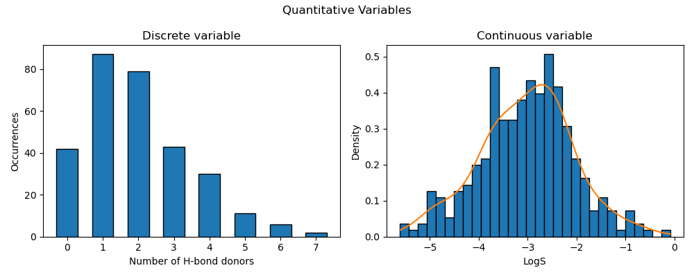
Quantitative variables generally split into two categories.

1. Discrete: The values jump from one number to another rather than spanning the full numerical spectrum in between.
   • e.g., counting the number of people in a room. It will always be strictly natural (i.e., positive integers) because there are no such things as 0.5 individuals.
2. Continuous: The values span the whole spectrum of an interval.
   • e.g., temperature in °C. A temperature can be 25, 25.2, 25.58, etc. All real values between any two intervals are possible.

The importance of understanding this distinction in quantitative variables lies in determining which math one can use: discrete mathematics (extended beyond qualitative variables) or calculus.

Discrete variables still resemble qualitative variables in a sense. They still capture a variable in terms of pieces (e.g., instead of low, medium, high, … it becomes 1, 2, 3, …), but with added functionality. Now, one can do mathematical operations like addition, subtraction, or division, and the result will be producible and meaningful.

For continuous variables, it becomes intuitive to use calculus concepts like derivatives and gradients. For those familiar with machine learning lingo, and especially deep learning, these words are a buzz.

Another categorization of quantitative variables, which can work with both discrete and continuous categories, is:

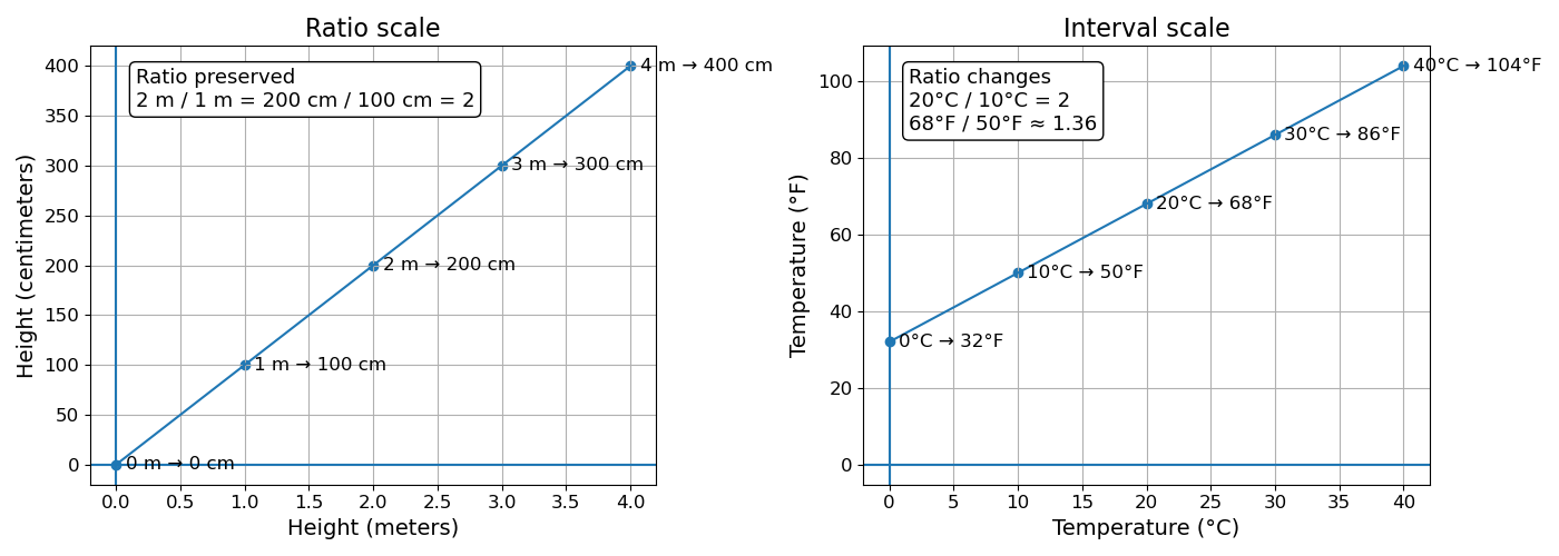
1. Ratio (scale invariant): The values lie on a scale where zero is a true zero and means “none of this thing.” Therefore, ratios are meaningful.
   • e.g., a tree that grows from 1 m to 2 m has “doubled” in height. This doubling means the same thing regardless of the unit used to measure height (e.g., centimeters, feet, or inches).
2. Interval (scale variant): The values lie on a scale with equal spacing but an arbitrary zero point. The zero does not represent “none of the thing”—it is simply a chosen reference. As a result, ratios are not meaningful.
   • e.g., for temperature, on the Celsius scale, zero means frozen water, not “no temperature.” If I have a temperature of \(10^\circ C\) and I want to “double” the temperature, this does not have a clear meaning because \(10^\circ C\) does not mean 10 units of heat; it merely means 10 units away from the arbitrarily chosen reference. So, performing an equation like \(2\times20^\circ C\) does not double the temperature; it doubles the distance from that reference point.
   • To anchor the meaning in different scales, \(20^\circ C / 10^\circ C = 2\), but the same temperatures expressed in Fahrenheit become \(68^\circ F / 50^\circ F \approx 1.36\). The meaning of the ratios is not anchored because the scale is arbitrary.

Differentiating between when a variable is ratio or interval is also important in determining which level of math is possible to apply. Any math that requires a clear and correct definition of zero, and therefore ratios, will not be “intuitively applicable” to an interval variable (e.g., proportions, exponential functions, and logarithmic functions).

Different types of relationships (functions)

Now that I know my variables, the next step is to know my “relationships.” In the field of mathematics, this is well known by the name of “functions.”

A relationship is established between at least two elements; here, it will be two variables. And following the traditional lingo, they will be named X and Y. A function is the relationship that will show me whether there is a way to map from the variable X to the variable Y. The traditional equation is

\(Y\) and \(X\) represent the full variables with all possible outcomes, while \(y\) and \(x\) represent specific values of the variables.

E.g., \(Y=[2, 4, 8, 10]\) and \(X = [0.2, 0.4, 0.8, 1]\). Then the relationship between any pair of values in both variables (e.g., \(y=2\) and \(x=0.2\)) is 10 (i.e., \(y = 10x\)).

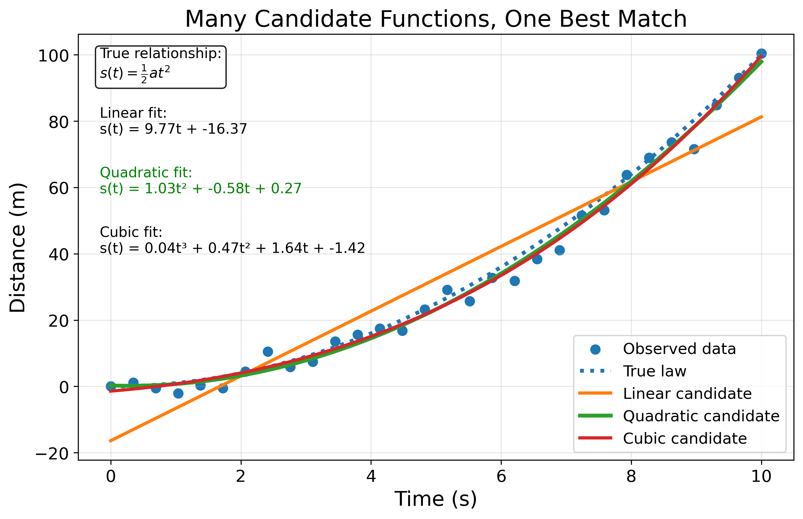
The goal everyone chases in the fields of mathematics, statistics, and supervised machine learning is to find the “right” \(f(x)\) for a given \(y\). The candidates for such a function can be vast (Figure 4), spanning linear relationships²:

Non-linear relationships:

Or a mixture of linear and non-linear relationships:

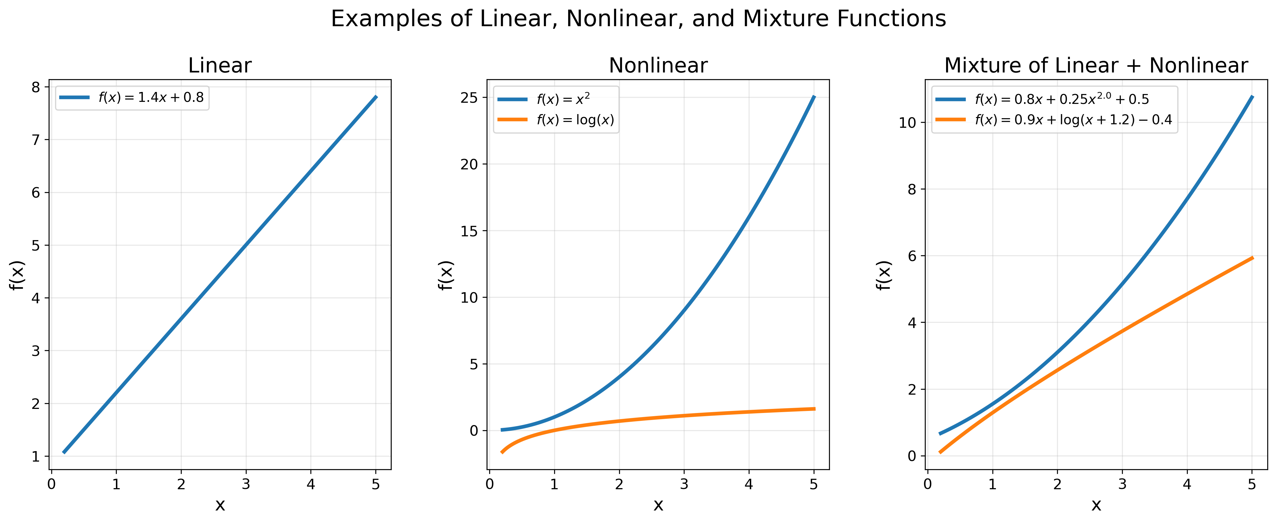
The way to decide which function is the “right” one for a given \(X\) and \(Y\) is to plug in each \(x\) and \(y\) and see which function gives the (almost) right answer. Check Figure 5 for a simple example of competing functions describing the displacement equation.

While the exploration space of \(f(x)\) can span infinitely many shapes, the type of the variables can help limit this space. This limitation starts by defining whether both variables share the same type (e.g., both nominal or both continuous), or whether they differ from each other (e.g., \(X\) is nominal and \(Y\) is continuous).

\(X\) and \(Y\) are the same

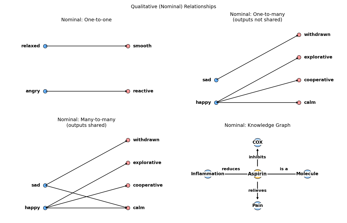
If both variables are nominal, for example, then the function will be rule-based (i.e., if \(X=x\) then \(Y=y\)).

These rules can also come in different flavors: one-to-one mapping, one-to-many, or many-to-many. And if the number of variables is higher than two, one can start drawing a graph and connecting the concepts like a mind map. Check Figure 6 for visuals.

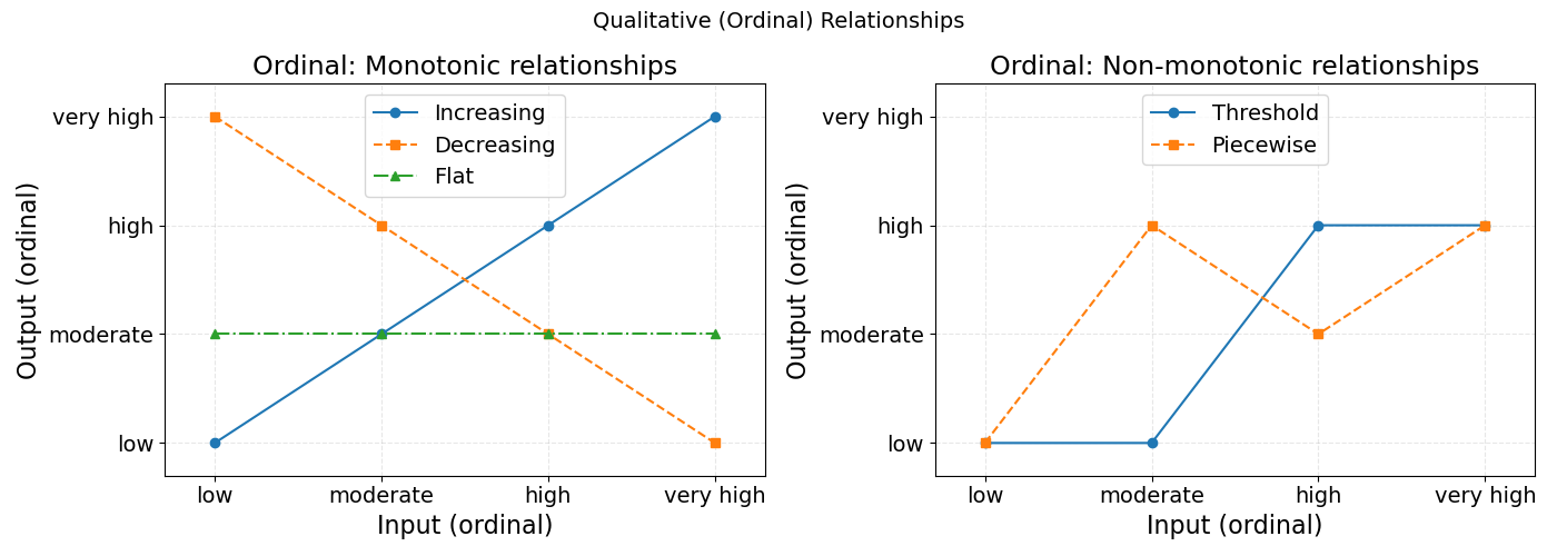
If the two variables are ordinal, then values have a specific order of appearance, and this changes what the relationship can look like. Now, relationships move from rule-based to threshold-based (e.g., if \(X<x\) then \(Y \ge y\)).

The ordering also allows for monotonic relationships, where the two variables can increase/decrease together or against each other. Check Figure 7 for visuals.

If the two variables are quantitative, one has two categories, discrete and continuous, and two subcategories, interval and ratio.

Discrete interval variables expand on ordinal variables by having equal spacing (i.e., distance), which allows for additions and subtractions. This further allows for arithmetic operations like deviation (i.e., subtracting values from the mean) and covariance (i.e., checking whether deviations move together).

I tried to find two variables that are discrete and interval put into a relationship together, but I could not find a meaningful or interesting example. So, I will speak about two interval variables, generally either discrete or continuous.

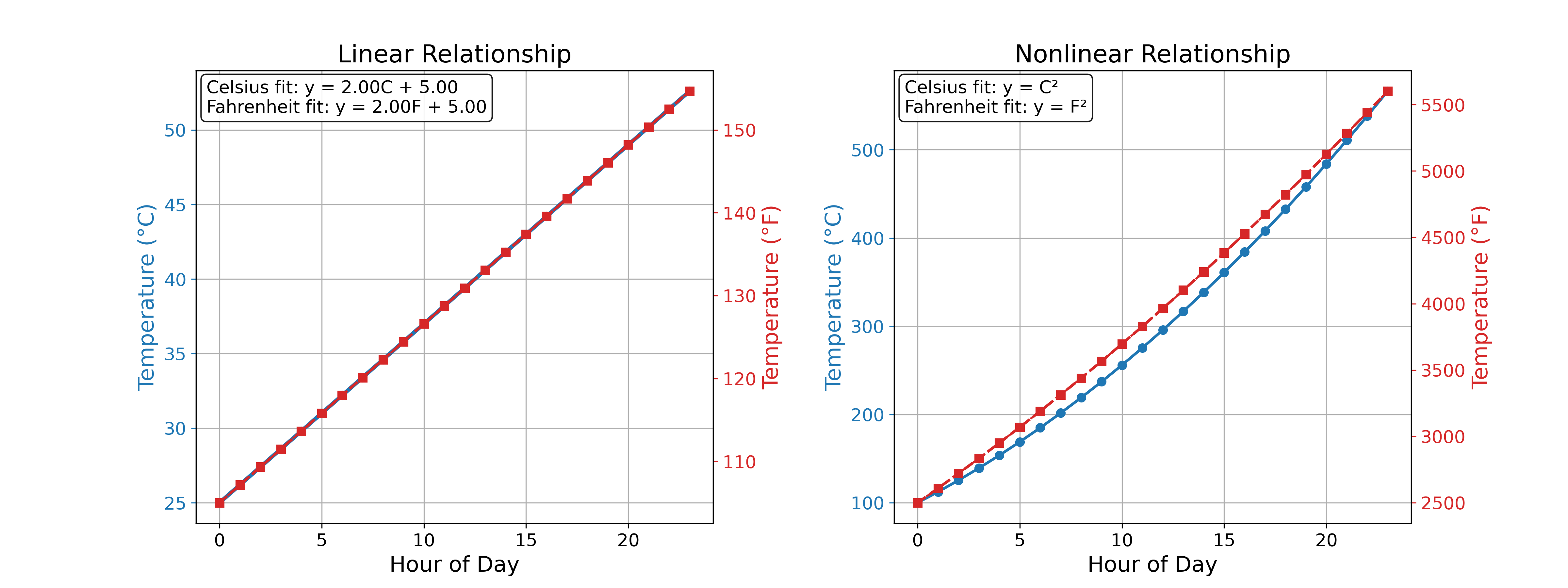
These interval variables are most naturally interpreted through linear functions such as \(y = ax + b\). This equation simply says that if \(X\) were a differently scaled version of \(Y\), it would be scaled by the factor \(a\) and shifted by the offset \(b\). This is exactly the case between the Celsius and Fahrenheit temperature scales, for example (\(C = \frac{5}{9}(F - 32)\)).

However, a function like \(y = ax\) or \(y = x^a\) or any other non-linear function would fail to produce a meaningful result without caution. This is because these functions rely heavily on the value of \(x\) having an intrinsic meaning, which makes manipulating it also meaningful. However, since the scale of \(X\), and therefore the values \(x\), is arbitrary, they are not easily manipulated in a meaningful way.

Recall the temperature and height examples in Figure 3: doubling the temperature on the Celsius scale is not the same as doubling the temperature on the Fahrenheit scale. However, doubling the height on the meter scale is the same regardless of any other ratio scale used.

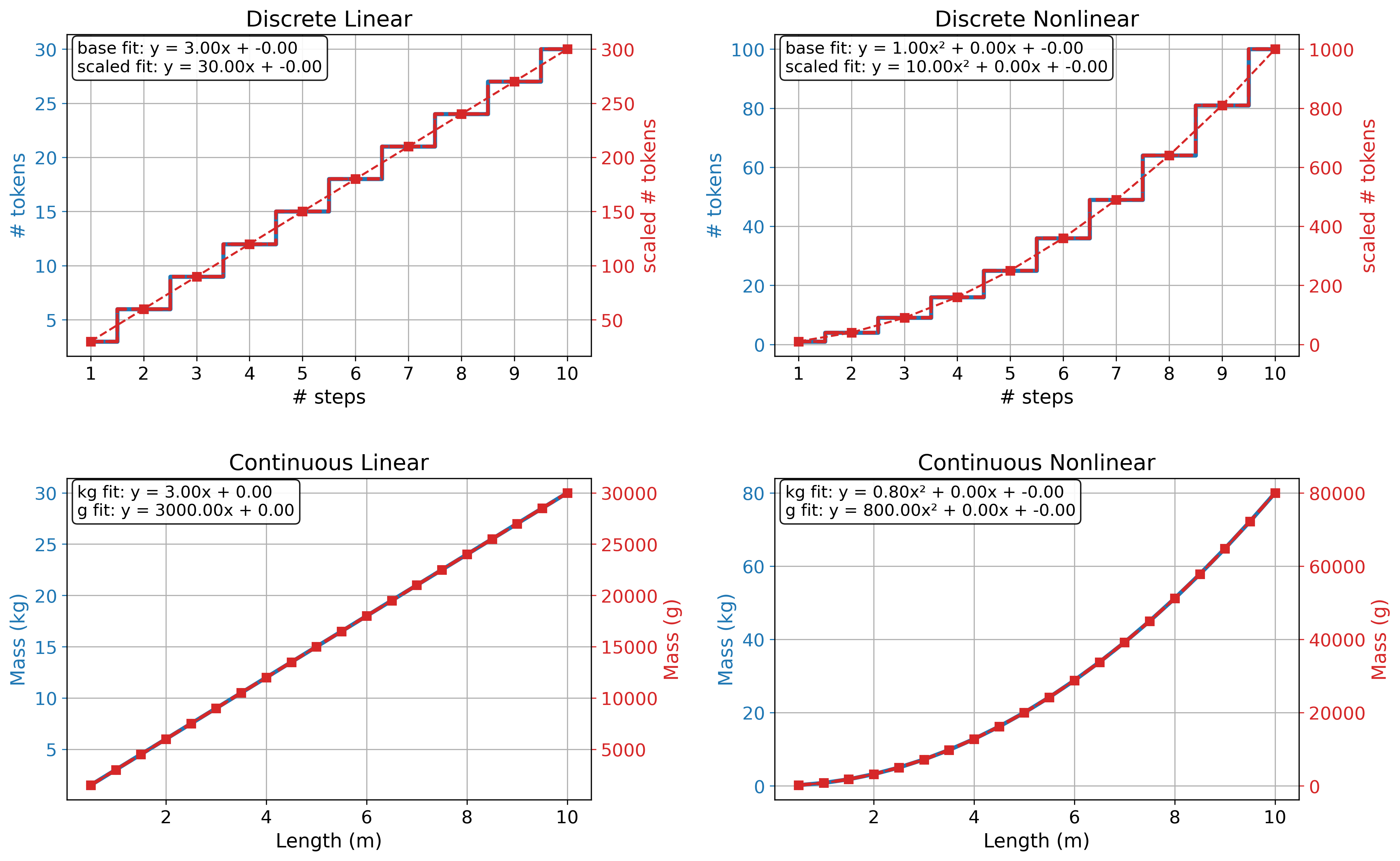
Figure 8 further reinforces this distinction with an example of how a linear relationship preserves the meaning between two interval scales while a nonlinear relationship diverges.

To relax the strictness of “non-linear transformations are not meaningful,” one can say they are, under strict and clear communication of the meaning of this transformation.

1. Clearly communicate that the transformation is meaningful only from the arbitrarily chosen reference, not from the value itself.
2. Clearly communicate that the transformation is strictly valid for this scale, not any other.

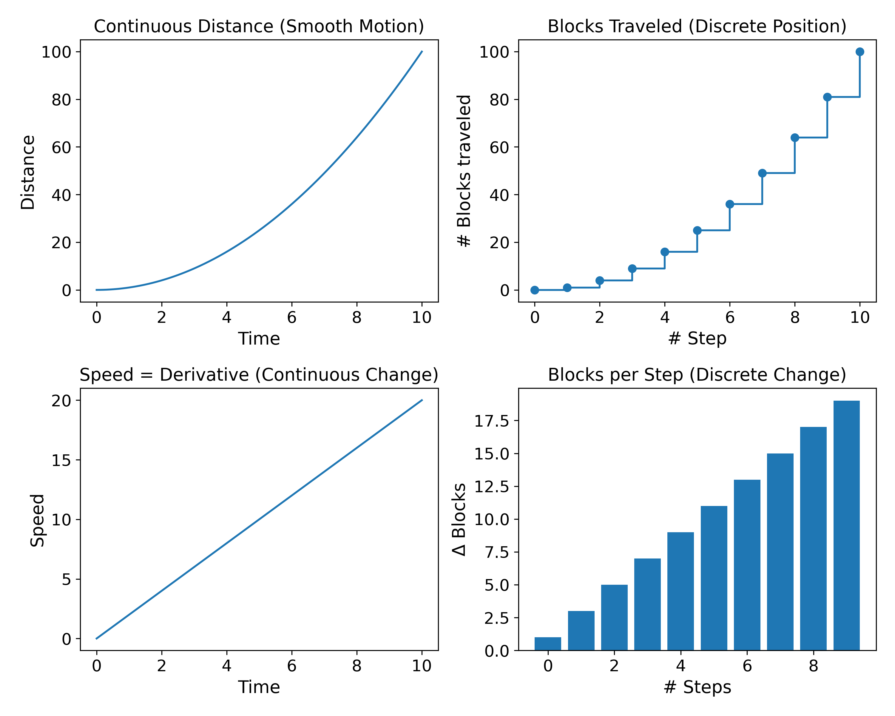
Continuous interval variables follow the same rules (i.e., additions, subtractions, linear relationships), but the difference lies in how changes are expressed mathematically (Figure 9).

For discrete variables, accumulation is represented by summation \(\sum_{i=1}^{n} x_i\) whereas for continuous variables, accumulation is represented by integration \(\int_a^b f(x)\,dx\).

Similarly, change between discrete points is expressed with simple differences such as \(\Delta y = y_{i+1} - y_i\) whereas continuous change is expressed using a derivative \(\frac{dy}{dx} = \lim_{\Delta x \to 0} \frac{\Delta y}{\Delta x}\).

Thus, discrete interval variables typically lead to difference equations, while continuous interval variables allow the use of differential equations, including derivatives and integrals.

If the two variables are discrete ratio or continuous ratio, then the function can safely take other shapes with meaningful interpretations, like proportions (i.e., \(y = ax\)), exponential (i.e., \(y = x^a\)), logarithmic (i.e., \(y = \log(x)\)), or any other transformation.

The difference between the two variables remains in the sense that a discrete ratio variable will stick to discrete math, while a continuous ratio variable will allow calculus (Figure 10).

\(X\) and \(Y\) are different

If the variables differ from each other in type, this leads to interesting cases because, as I have explored, each variable allows for certain functions. When variables agree, the math used is unified, but what happens when they disagree? Would the math still work seamlessly?

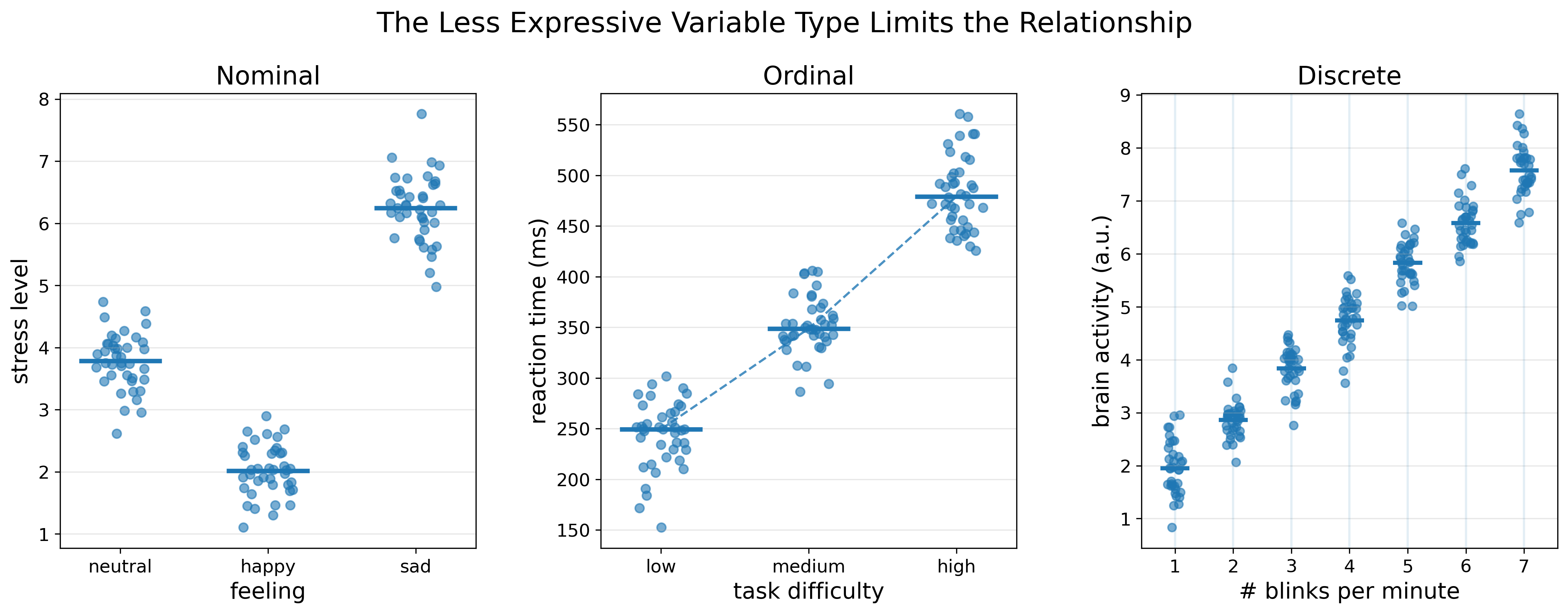
Short answer: when two variables interact, the mathematical relationship is limited by the least expressive variable type (Figure 11).

The easiest case, in my opinion, is when one variable is nominal and the other comes in any shape. Because nominal variables are the most restrictive of all types.

Once a variable is nominal, it already divides the other variable into spaces, and nothing more can be done.

For example, if \(X\) = feelings (i.e., nominal) and \(Y\) = stress level (i.e., ordinal), \(Y\) will immediately get distributed over \(X\) in a mixture of rule-based and threshold-based functions (e.g., if \(X=x\) then \(Y>y\)).

If \(Y\) = FMRI activity (i.e., continuous) or number of blinks per minute (i.e., discrete), the same thing will happen, except that the description of the \(Y\) splits can be more expressive. E.g., if \(X=x\) then \(Y \in [a, b]\) where a and b are the minimum and maximum values of the subset of \(Y\) under a given \(x\). Or if \(X=x\) then \(Y=\mu\) where \mu is the average of the values that fall under this \(x\).

So, nominal variables restrict the function to being rule-based, and allow flexibility only in how one chooses to describe the distribution of \(Y\) over \(X\).

The case where one variable is ordinal, and the other is quantitative is very similar to the nominal case. The ordinal variable splits the quantitative variable into spaces as well, with the only difference being that the spaces are ordered. E.g., \(\text{median}(Y \mid X=\text{low}) < \text{median}(Y \mid X=\text{medium}) < \text{median}(Y \mid X=\text{high})\).

The same happens when one variable is discrete and the other is continuous, although this case can easily trick the observer. In this case, both variables take ordered and equally spaced values, which makes them look very similar to each other. However, discrete variables still jump on the number line rather than covering it smoothly. This means that one cannot safely perform derivatives or gradients on them, and they will end up splitting \(Y\) into spaces, just as nominal and ordinal variables do.

\(Xs\) and \(Ys\)

So far, I have been contemplating the case of only two variables. But the problem is notoriously bigger than this.

In supervised machine learning, the typical setup is that one has multiple \(Xs\) to infer \(Y\) from. The equation is

If the setup is multi-task learning, then one has multiple \(Ys\) as well, and the equation becomes

In the previous two headers, I discussed how \(X\) and \(Y\) interact in different ways, but now the interaction happens at a bigger scale.

Each \(X_i\) can indeed still interact with \(Y\) in the ways specified, but now each \(X_i\) can also interact with another \(X_j\) (including itself) to affect the result for \(Y\).

The bigger function \(y = f(x_1, x_2, \dots, x_n)\) can be broken down into the same linear, non-linear, and mixed functions specified at the beginning of this section.

But now one also considers the linear, non-linear, and mixed interactions between every two or more variables.

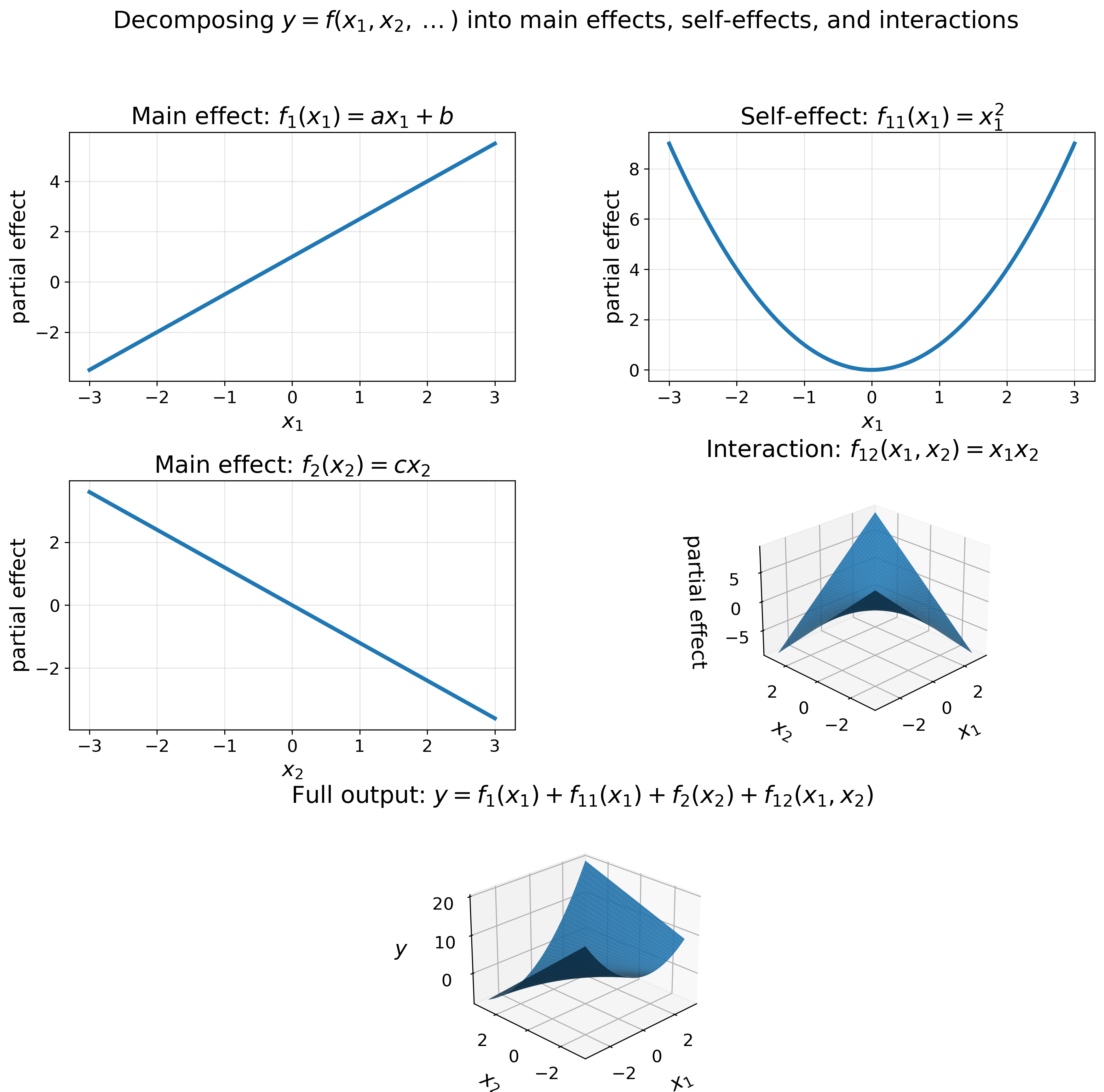
For example, considering two interacting variables \(X_1\) and \(X_2\) influencing \(Y\), the function \(f(x)\) gets expanded into shapes like the following:

All these possible functions compete together as an accumulation, and the surviving functions get to make the final function for \(Y\):

Where each \(f_i(x)\) represents one possible relationship and \(w_i\) corresponds to the weight of this relationship in affecting the final output of \(Y\). Similar to Figure 5, the data chooses which relationships survive and with which weights.

Figure 12 below shows how different transformations influence the prediction of \(Y\), and how the final relationship between \(X_1\), \(X_2\), and \(Y\) turns out.

With such an explosion, the human is no longer capable of mindfully staying in the loop, and the task gets delegated to a machine with powerful memory designed for the task.

Even when the machine is powerful, if the size of \(Xs\) spans from hundreds to thousands, exploring all possible relationships can still be infeasible.

When the number of variables and the possible interactions between them explodes like this, it becomes even more important to keep track of the variable types. This will be one’s guardrail for limiting this explosive space.

One can introduce rules or algorithms to identify and respect the type of each variable and the math it gets access to.

For example, the nominal variables within \(Xs\) become default limiting factors because they inevitably split the space of any other variable they interact with, and one cannot do anything about it. If such nominal variables are indeed important for understanding the problem, then one is bound to respect how they split the space of the other variables.

If a variable is nominal or ordinal but takes the shape of a discrete variable, such as replacing low, medium, high with 1, 2, 3, this can be tricky for both the observer and the model. The latter gives the notion that \(2-1=1\), but in reality one does not know what the result of medium - low is.

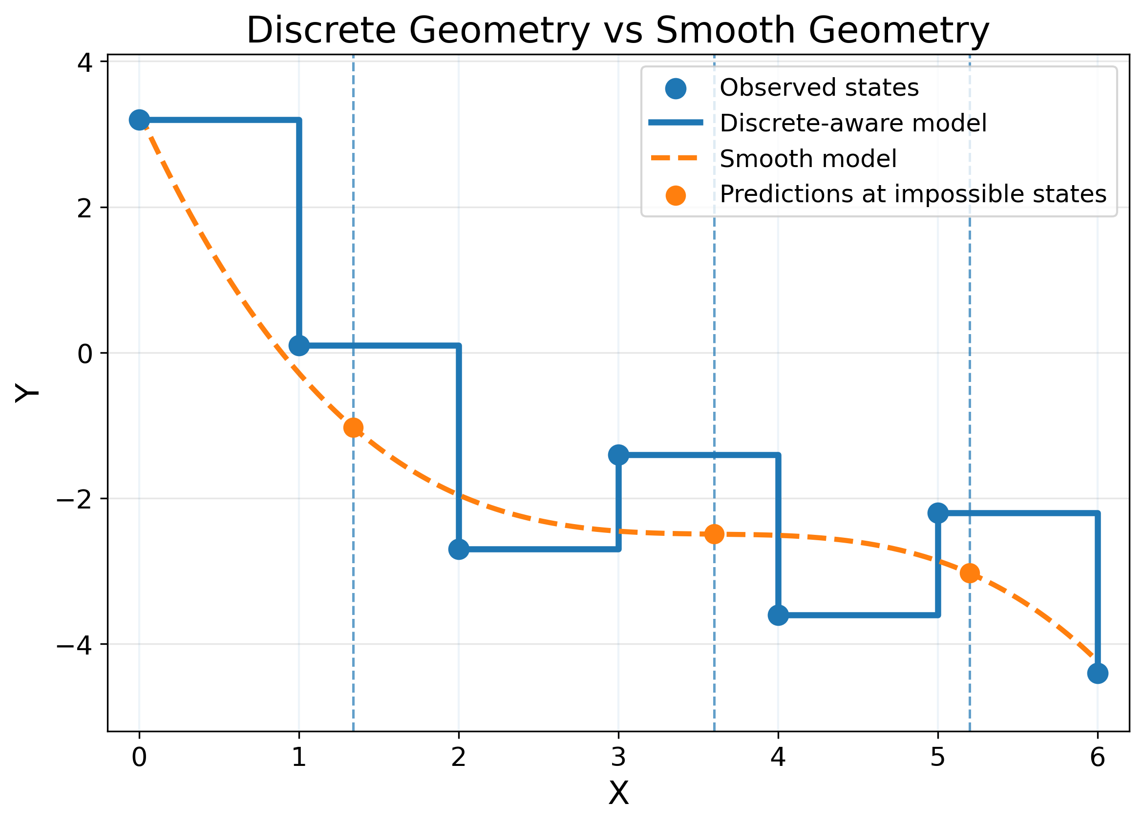
If a variable is discrete, one needs to be careful when applying calculus to it because many models that deploy calculus assume continuity and smoothness.

The continuity assumption leads to learning functions where it is possible for a discrete variable to take a value like 1.34, although this is not possible. This artifact might or might not be harmful.

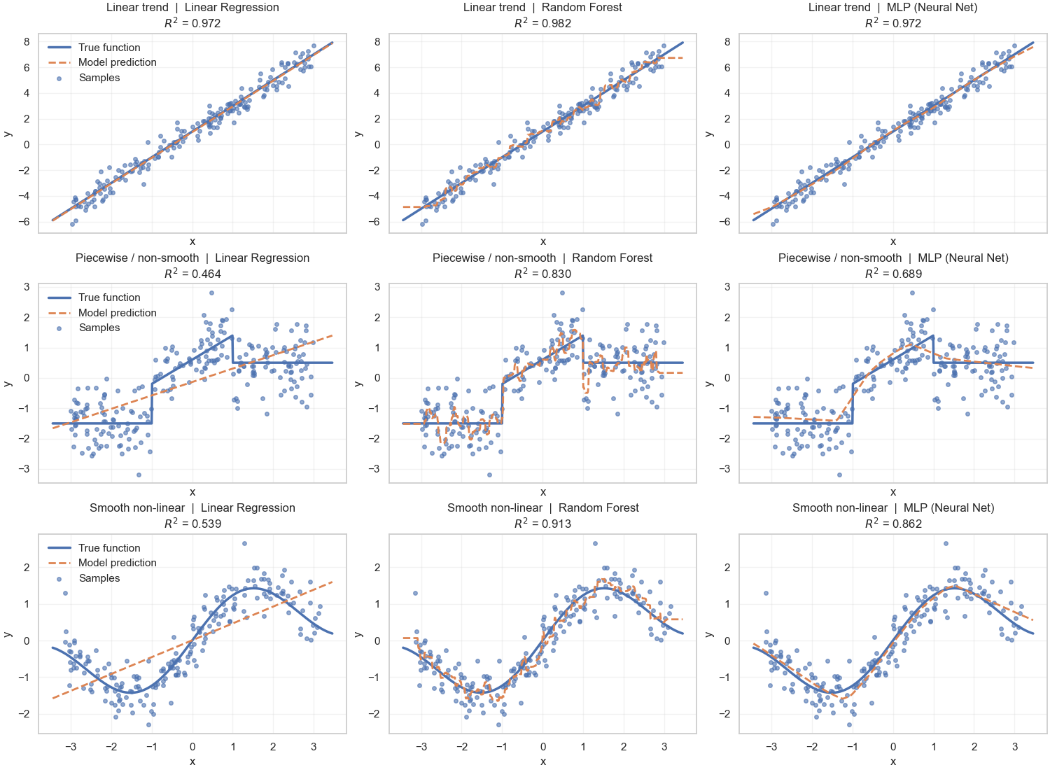
Smoothness assumes that points in a variable near each other must lead to similar effects on another variable, but the jumping nature of the discrete variable can encode abrupt jumps in another variable. A smooth function will punish such jumps even though they represent the truth (Figure 13).

In this section, I am mainly concerned with how the type of variables can shift my thinking about which model to use. And it led me to realize that it is about variable geometry.

Most current machine learning algorithms (as will be discussed in a later post) rely on Euclidean geometry, which is the geometry of continuous variables. Yet the reason that got me into this topic initially was realizing that most of the variables I deal with in my PhD work are not continuous!

Different worlds of functions (frameworks)

Besides the types of variables affecting what math a function can use, there is still another factor that shapes what it can look like.

This time, the factor is related to the conceptual framework of the person searching for it. It is what this person assumes about this function, and therefore how to approach it.

I came to think of these frameworks as defining different views of the same function. Two of them are fundamental: deterministic and probabilistic, and the rest follow from them but with additional conceptual assumptions: causal, predictive, generative, and agentic.

Deterministic frameworks

In the deterministic view, the researcher has an assumption about the problem, an assumption of structure.

The researcher “believes” that there is a unifying force tying the different variables of the problem together and leading to a deterministic function with a single outcome for each value.

Here, \(y\) will always have one and only one corresponding value for each input \(x\).

It also assumes that all variables needed for this structure are attainable; thus, the function itself is attainable.

To make this distinction clear, in another framework, the function will take the form

where \(\epsilon\) is a probability distribution representing the possibility of missing variables or mismatched assumptions.

In deterministic frameworks, one has already made the assumption that there must not be an \(\epsilon\).

The researcher’s job then turns into figuring out how to land this function.

As far as I can comprehend, this setup will mostly be applicable to physical and natural laws that one stumbles upon rather than contributes to. I can think of three setups leading to such deterministic functions:

1. One designed the system themselves, and thus they assigned the function already (e.g., a simple case of a professor mapping exam grades from percentages to letters, or a more advanced case of someone developing their own algorithm).
2. One has large i.i.d. data that is representative of a problem and covers all its facets, such that one can now find the function that describes this problem perfectly (e.g., calculating the circumference of a circle; initially, people did it empirically until the data hinted at the equation \(y = 2\pi r\)).
3. One was inspired by a formula for how something works, and when it was applied to its context, it always gave the desired result (e.g., Newton’s second law or Einstein’s relativity equations).

Probabilistic frameworks

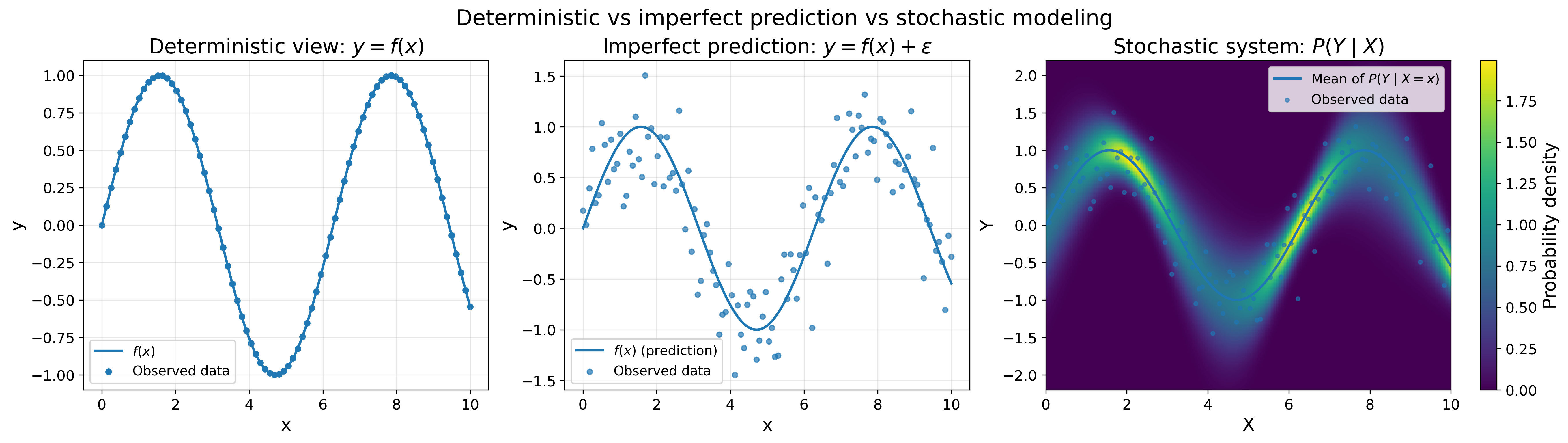
In the probabilistic view, the researcher accounts for cases where the system is missing components, and thus the answer is not reached perfectly but only partially:

Or the system itself is stochastic, meaning it does not give the same answer under the same observable conditions. In such cases, one calculates a probability distribution for the outcome \(Y\) given the current knowledge \(X\).

This reads as follows: given \(X=x\), what are the possible values \(y\) to observe in \(Y\)? Figure 14 shows the difference between the deterministic view and the probabilistic view in its two facets: imperfect prediction and true stochasticity.

In this framework, one moves away from the certainty assumption in the deterministic framework and toward a system of uncertainty. I can think of the following cases where uncertainty is in the system, and thus probabilistic frameworks are more suited to it:

1. The measurement of the variable \(Y\) is noisy. Therefore, even if the relationship is deterministic, one does not have the appropriate data to find it. In such a case, one knows that the goal is not to output a single value of \(y\), but rather an uncertainty measure around it (i.e., \(P(Y \mid X)\)).
   • One example from chemistry is experimental procedures that rely on multiple factors, from well-calibrated equipment and well-maintained materials to well-handled execution, and even to the original assumption about the validity of the measuring process itself. When these steps are not accurate enough, we end up with noisy data, and the same measurement for a compound is not reproducible across experiments. Therefore, the function used to map this relationship would also respect this uncertainty and infer probabilities rather than single values.
2. The variables \(X_1, X_2,\dots, X_n\) used to infer the outcome \(Y\) are not suitable or are incomplete. In such cases, the relationship between \(X\) and \(Y\) can only be approximated to the best allowed by the information provided by \(X\) (i.e., \(y = f(x) + \epsilon\)).
   • The never-getting-old example from cheminformatics is the struggle to find sufficient representations for our molecules. I recall Tony, the medicinal chemist postdoc in our group, once telling me in a discussion that chemistry is the science of the electron. If one finds the right functions to calculate the quantum states of electrons, one has chemistry figured out. But because we are not there yet, we can only represent molecules using variables that approximate these quantum functions, probably not in a great way.
3. The function \(f(x)\) used to map between \(X\) and \(Y\) is not appropriate. This happens when one uses the wrong assumptions about the relationship and ends up measuring or approximating it using an inappropriate, or simply less ideal, function (i.e., \(y = f(x) + \epsilon\)).
   • This was shown in Figure 13 when a smooth function was used to model a non-smooth relationship. The smooth function will be close to correct in some places, and completely off in others.
4. The system itself is truly stochastic. It is not about noisy measurements, missing variables, or mismatched functions. The system gives different answers even if the observable conditions are the same (i.e., \(P(Y \mid X)\)).
   • This is, of course, a very well-known phenomenon in quantum mechanics, such as calculating the position of an electron. One cannot determine the exact position of an electron, but rather the probability of finding an electron at some position.

I can think of another case that would conceptually fit this framework, but with a caveat, in my opinion.

• The variables \(Xs\) and/or \(Y\) do not span the full range of their possible outcomes, making the data incomplete.
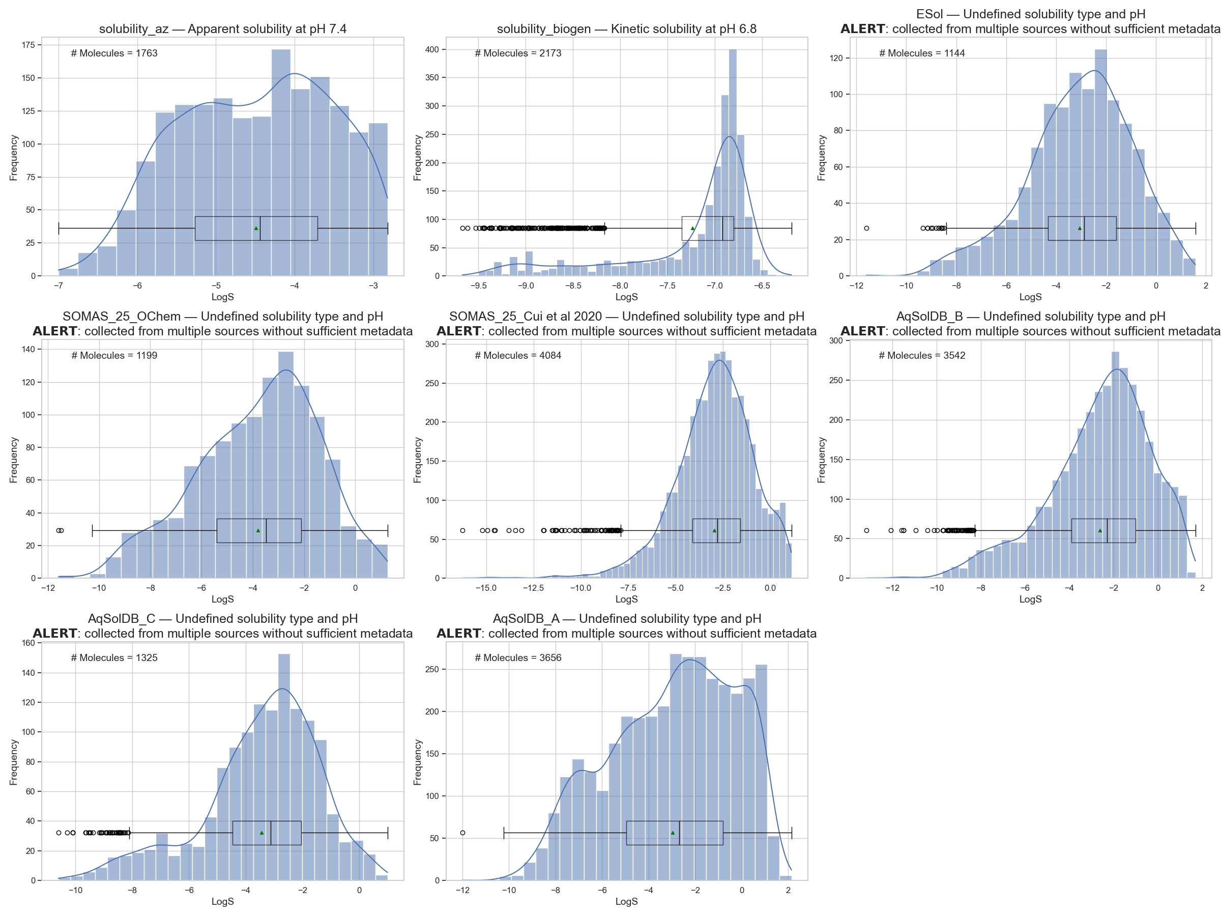
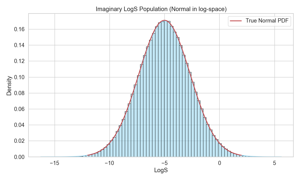
  • A loose example could be the relationship between molecular weight and aqueous solubility measured in LogS. Molecular weight can range from \(<100\) to \(>500\) daltons. If one measures LogS for light molecules only, one may find a linear relationship, but as the molecular weight increases, the relationship might start becoming non-linear.

This case contains incompleteness, as in the missing-variables or mismatched-assumptions cases. However, the incompleteness would be relevant only if one decided to use the function fitted on this specific range of both variables to infer other ranges.

Incompleteness is not inherent to the function or the data, but rather to how the person applies the function in the future.

Causal frameworks

Causal frameworks are concerned with the mechanics of the relationship; they ensure that a relationship, deterministic or probabilistic, is obtained for the “right” reason.

To explain what “right” reason means, I feel like I need to split the framework into two phases: pre-data-explosion and post-data-explosion.

In the pre-data-explosion phase, data was scarce and costly, obtained through a carefully designed experiment to measure variables of interest. Only after collecting data could one attempt to find the function describing the relationship between such variables.

The next question would intuitively be: which variables should be measured?

Depending on the task’s difficulty, a researcher can have freedom in the variables to choose from. But I would assume that any experiment requiring human labor would eventually call for careful consideration to make the measured variables as relevant as possible to the problem under investigation, and as variables that are “believed” to be instrumental to it.

This “belief” is at the heart of the causal framework for this phase. A researcher relies on prior established knowledge, or on their own expertise stored in their brain or gut, to select the variables \(X\) and \(Y\).

Once \(X\) and \(Y\) are selected, one performs a scientific experiment to generate data that would help find the function linking them together.

This experiment would follow the good old scientific principle:

1. Intervene by changing \(X\) to one’s desired value.
2. Watch whether \(Y\) changes as \(X\) changes.
3. Pay attention to confounding factors to the best of one’s knowledge and experience (i.e., an uncontrolled third variable \(Z\) that might be the main reason behind the change, not \(X\)).
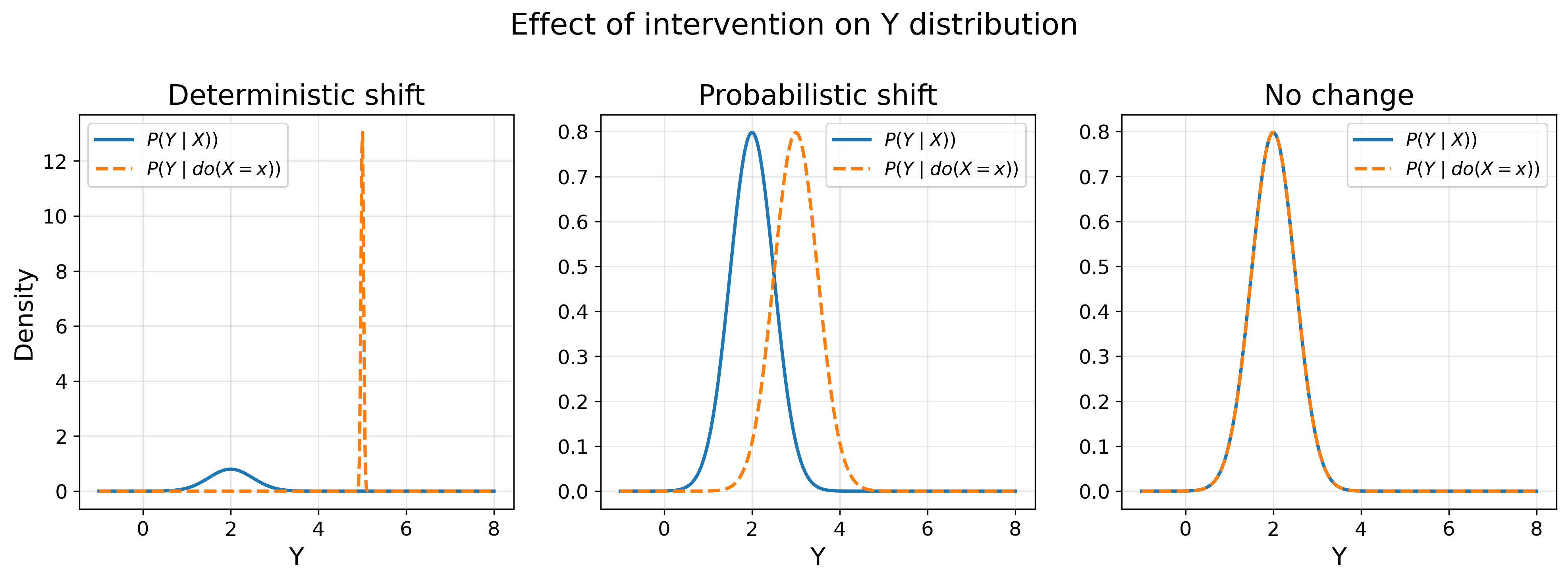
4. Examine the change in \(Y\) to judge whether it is enough to conclude a plausible relationship with \(X\) (i.e., \(P(Y \mid do(X))\)) (Figure 15).
   • If changing \(X\) leads to the same change in \(Y\) every single time (i.e., \(P(Y=f(X) \mid do(X)) = 1\)), then a causal relationship is established, and the relationship is deterministic.
   • If changing \(X\) leads to a distributional shift in \(Y\) (i.e., \(P(Y \mid do(X)) \neq P(Y)\)), then a causal relationship is established, and the relationship is probabilistic.
   • If \(Y\) does not change (i.e., \(P(Y \mid do(X)) = P(Y)\)), then the relationship is not established, and the experiment is open for exploration again.

Once \(X\) is established to influence \(Y\), one can then start searching for the function (deterministic or probabilistic) that models this relationship.

In the post-data-explosion phase, the scene changes as follows:

1. A statistician starts with loads of already measured or calculated variables that might or might not be instrumental to the problem.
2. A plethora of functions can be applied to different variables to establish relationships between them.
3. The researcher ends up with the best function to describe how \(X\) relates to \(Y\).

But one needs to always remember the never-old wisdom:

Correlation does not imply causation

One can have two variables and find a function that describes them (almost) perfectly, but without a “logical justification” as judged by an expert on the problem.

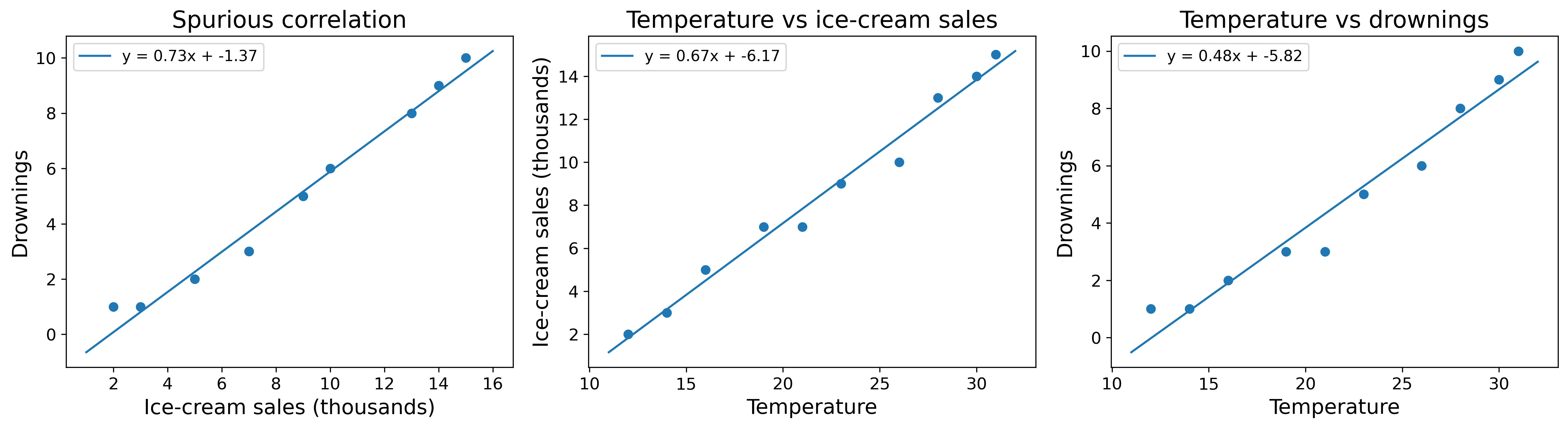
A very famous example is the number of ice creams sold per month (which I will call \(X\)) versus the number of drownings in the same months (which I will call \(Y\)).

The relationship turned out to be \(y = 0.73x-1.37\) (Figure 16). Meaning, if one knows the ice cream sales of a month, one can predict how many drownings will occur.

But I hope one can easily stop and say: Wait a minute! I do not understand what would make ice cream sales relate to drownings! Is something missing?

And indeed, the missing piece was a third variable, \(Z=\text{temperature}\). Temperature turned out to be a confounding factor that explains how ice cream sales and drownings could have been related.

Higher temperatures call for more ice cream consumption as well as more swimming. More swimming leads to more possibilities of drowning.

So, if one was interested in understanding the main cause behind drowning and used ice cream sales instead of temperature, one would find a perfect function to tie them together.

But it was the human’s judgment of the physical and experiential world that made this relationship die in its infancy even though it perfectly described the observed data.

Therefore, a causal framework can be thought of as the framework of strong assumptions. A relationship is not permissible without validation of a logical connection between the variables.

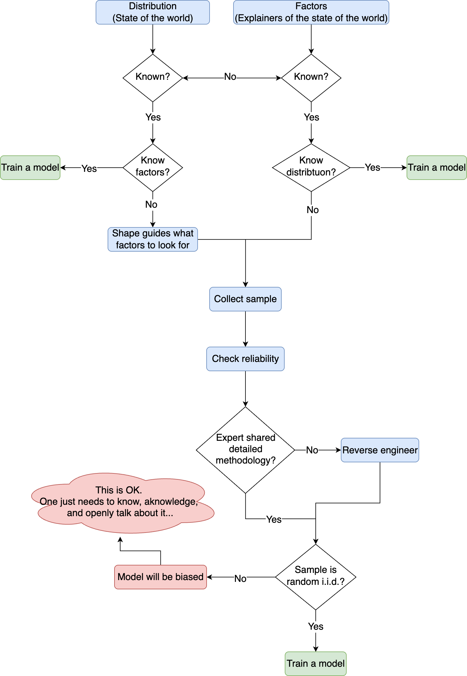
To ensure causality in the data-explosion era, one would be bound to rely on the expert’s assumptions about a problem to:

1. Spot whether some variables are confounding.
2. Spot whether policies and practices led the data to look the way it did, rather than reflecting an honest view of reality.

These assumptions can then be formalized in explicit algorithms that scan the data to find them and handle relation permissibility through logic.

One example of such algorithms is causal graphs. In this algorithm, logical relationships get encoded in directed acyclic graphs (DAGs) that help determine confounding factors.

In the drowning example, if one used the variables \(X_1=\text{ice cream sales}, X_2=\text{swimming}, X_3=\text{temperature}\) to predict the variable \(Y=\text{drowning}\), the DAG for this problem would look like this:

Temperature → Ice cream sales

Temperature → Swimming → Drownings

And this graph would label temperature as a confounding factor.

Predictive frameworks

In this framework, one realizes the slow nature of the causal framework relative to the amount of data available nowadays, dislikes it, and decides to change it.

The predictive framework tries to answer a single question: does this data help me make good predictions about the future?

At first glance, this question might not feel that different from the other frameworks. If one suspects causality and finds the relationship, then one can easily predict the future within the certainty level of that relationship.

So, where is the novelty?

Well, in the causal framework, one needed to emphasize the phrase correlation does not imply causation and use it as a safeguard to filter “spurious” relationships.

But in the predictive framework, one need not worry about spuriousness.

In the predictive framework, if a relationship works well enough to predict the next outcome, one accepts it, celebrates it, embraces it, and moves on. DO NOT SEARCH FOR LOGIC!

Predictive frameworks are not meant to spot or explain logic; they are goal-oriented, where the end justifies the means.

They try to find the same probabilistic function as before:

The only difference is that now \(X\) represents whatever variables one has rather than a “carefully curated set of variables” (Figure 17).

To make this more tangible, remember the ice cream sales versus drownings example. A human was not satisfied by this relationship because it did not make sense given physical and experiential logic, which made them look for a “more plausible” connection to drowning.

But the thing is, if predicting drownings was the goal, then ice cream sales do predict it.

As long as people buy more ice cream and swim more as the temperature gets higher, the relationship between ice cream sales and drowning would still work.

The only thing to change would be our intellectual satisfaction as human beings, not the result.

So, the predictive framework does not provide changes to the mathematical or functional world, but rather an epistemological and philosophical stance.

The predictive framework forces one to think about the end goal, because this end goal is the only thing that determines which route to take!

• If my end goal is to satisfy my curiosity by understanding the mechanics of the problem, then I will use causal frameworks.
  • It is slower, and requires lots of communication between experts, but this is the road to “understanding.”
• If my end goal is to manipulate the system and tweak it to my desire (e.g., optimizing a molecule for drug development), then I will “eventually” need to “understand” the problem. Then I might use either the causal framework only, or a mix of causal and predictive frameworks.
  • This mixing would usually happen by starting with causality, using it for predictability, learning something new about the system, integrating it into the causal framework, using it again for predictability, and repeating.
• If I trust the system to be static and well-behaved, and I am interested in working around it rather than understanding or manipulating it, then predictive frameworks are all that I need.

In my opinion, any attempt to start with a predictive framework and then post-hoc it for causality would be a needlessly redundant task.

When one tries to extract causality from predictive frameworks, one is basically doing the same work one would have done by using the causal framework from the beginning.

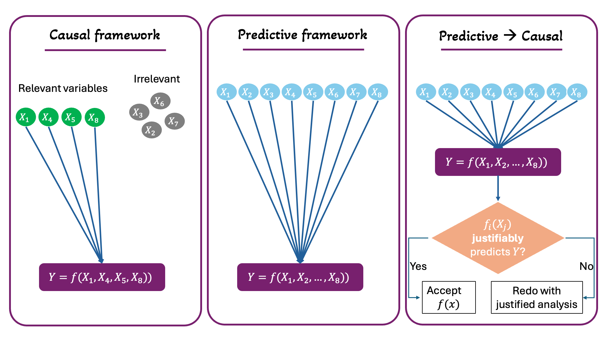
To make this redundancy clear, let us check this scenario. If one used 10 variables (\(X_1, X_2, \dots, X_{10}\)) to predict \(Y\), one has three options, and one of them is redundant (Figure 17).

1. The researcher performs sanity checks on these variables to see what is logical for predicting \(Y\), then selects only those for prediction → Causal framework.
2. The researcher uses all variables—without vetting them—to predict \(Y\) and simply trusts the process → Predictive framework.
3. The researcher uses all variables—without vetting them—to predict \(Y\), gets the relationships between each \(X\) and \(Y\), then checks whether each relationship is actually permissible → Predictive followed by causal (i.e., redundant).

Generative frameworks

In my opinion, a generative framework is a deeper version of predictive frameworks. It inherits the same guiding principle:

Trust the data and do not look for logic.

However, the task required of the model becomes significantly harder.

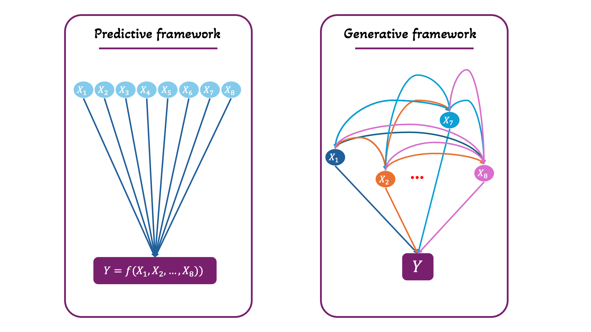
In predictive frameworks, the function to be predicted is \(P(Y \mid X)\); i.e., when one sees \(X=x\), what is the probability of seeing a specific \(y\) value from \(Y\)?

In generative frameworks, the function is

This is a joint probability distribution of the variables. The model does not only learn \(Y\) conditional on \(X\), but also each \(X_i\) conditional on the other \(Xs\).

In predictive frameworks, one only needed to find the function \(y = f(x)\), but in generative frameworks, one also wants to find all the functions \(x_i = f(y,x_{j \neq i})\) (Figure 18).

The goal of generative frameworks is to create a function that would reproduce the data, or generate new data that would look indistinguishable from the original. This comes from learning all bidirectional relationships in the data.

For example, one may have a dataset of molecules and corresponding aqueous solubility measurements. A generative model would learn all possible relationships between molecules, and between molecules and their aqueous solubility. Once this is achieved, a generative function can then generate new molecules with a desired aqueous solubility range.

While this framework feels powerful and flashy, one needs to be aware of the amount of possible spuriousness that can be propagated within it.

The predictive framework already relaxes the condition of logical consistency and allows for \(Xs\) to be redundantly or carelessly linked to \(Y\). Now, it additionally allows for \(Xs\) to be redundantly or carelessly linked to each other.

Because the model attempts to capture all statistical dependencies in the data, any coincidental or noisy relationships may be absorbed and reproduced by the model.

I will argue again that manipulating a system requires the implication of causality when intervening in it, if one wishes to walk in rationally grounded steps rather than irrationally independent ones³.

Here, in the generative framework, the goal is usually manipulation. It is to generate or simulate data similar to the original instead of producing it through labor.

Excluding causality relaxes the task and makes it easier and faster, but how far can one get while blindfolded?

Since generative frameworks have been exploding only recently, work on integrating them with causality is still in progress.

Agentic frameworks

I believe an agentic framework is the natural follow-up aspiration to the previous ones. If one has found a way to make functions that predict and generate, it becomes time to “delegate.”

The way I see it, there has always been a higher goal above whatever the previous frameworks were doing.

A causal framework tries to understand, a predictive framework tries to forecast, and a generative framework tries to reproduce reality.

But why are humans eager to understand, forecast, or reproduce systems?

I believe it has always been about control: controlling the environment, controlling the future, and eventually creating the environment and the future.

So, the end goal is not to understand, forecast, and reproduce. It is to use the knowledge and capabilities of these frameworks to propose policies and modifications to the system.

So far, the entity that uses this knowledge to propose policies and modifications has been strictly human. With agentic frameworks, one willingly delegates some of these decisions to an agent.

This agent operates within an environment defined by humans. It uses the data provided, explores the set of actions available to it, and proposes policies within the limits of the system it can observe and interact with.

The central question of agentic frameworks becomes: which actions should be taken to maximize a desired outcome over time?

Instead of predicting variables, the variables become a dynamic environment, and the agent must now learn a policy for action over different states of the environment.

The mathematical representation of this policy is

It reads as follows: given that the environment is in state \(s\), what is the probability of taking action \(a\)?

So, for agentic frameworks, one needs to provide a set of actions that would then be mapped to an environment. And the probability of each action will change as the state of the environment changes.

An example to lock this in can be a self-driving car.

• Agent = car
• Current state of the environment = a wall is approaching
• Possible actions = [turn left, turn right, brake]

The agent will need to assign a probability to each action given the current situation. These probabilities would be learned by generating different situations and environments and mapping which action gives the best results over time.

Again, an agentic framework feels magical, but still, as with each previous framework, the human is giving something up in exchange.

In predictive frameworks, humans gave up logical coherence.

In generative frameworks, humans gave up concrete goals (i.e., generate something similar synthetically rather than create something novel manually) and doubled down on logical coherence.

And here, in the agentic framework, humans are slowly letting go of their agency, their direct control over decision-making⁴.

The connection to ML and cheminformatics

While I have not discussed a single ML model like linear regression, random forest, or neural network, this post has made it much clearer for me to navigate such models.

The next technical post will focus on viewing such models in light of what has been discussed in this post.

Cheminformatics is an applied science branch that relies on advances in the ML field translating into advances in the chemical field.
However, this post also made it clear to me that transferability between the two domains is not as easy as one might think.

The math is general, but the application is strictly subjective to each problem, its variables, the relative knowledge available so far, and the researcher’s own goals.

In the next technical post, hopefully I will be able to explore how I shall think about applying ML models to a cheminformatics task after the current clarifications I went through.

I read The Tyranny of Merit by Sandel and started thinking about the feeling of not being valued as a member of society. A feeling that many blue-collar workers now experience, probably leading them to despair and worse.
I got to experience this fear myself, firsthand. I realized that I have been programmed to fear slipping into being a non-productive member of society in some stereotypical sense. I felt the need to make sure that I am useful in one way or another.

This is something that I am actively trying to reprogram myself from. I try to avoid seeing my value only through the lenses of society, and to be confident in my being as a value in itself. I need not perform to be absolved.
I believe that every human being has intrinsic value that no one should ever doubt, question, or demand to see proven on the spot.

And this got me thinking: the definition of value in our age, which Sandel calls “merit”, is an illusion. It’s a shared illusion that requires the participation of its members to hold.
And this meaning of value is ever shifting. In another place in the world, one’s value is in social generosity. In another time and place, it was being a Samurai. In another time, it was being a craftsman. In another time, it was being a farmer. And I think now my thought is clear.

So, if merit is an illusion that can be changed, and blue-collar workers are hurt by it, why not change the meaning of value themselves as well? The illusion holds because they are also participating in it.
So why wouldn’t those who are hurt the most by merit drop this illusion and make up their own? What is it that these people need but cannot make for themselves?

Then Tesla’s words hit me. Tesla, in his book My Inventions, saw himself as an inventor. His mother and father were also inventors in his eyes. He attributed invention to the most important core of a human being — the core that helps the human race evolve and survive.

But what was Tesla’s definition of invention? From what I gathered from his book, it was mainly engineering.

Tesla spent his life designing and creating tools. He praised his mother for being an inventor by planting her seeds, weaving her wool, and mending her house.
For Tesla, the human was an inventor (i.e., an engineer).

Becker, in his book The Denial of Death, looked at the human condition from the creative angle. A philosopher and psychologist whose task was to dismantle the human condition and make it explainable.

Becker did not mention a single engineer in his book, just as Tesla did not bother to think that thinking itself could be the end goal of invention.

Tesla and Becker made me think of two highly valuable and esteemed kinds of people in our current era who missed seeing each other as indispensable to one another.
The thinker cannot survive without the inventor inventing tools for survival and exploration. And the inventor could not invent those tools without others who decided to only think without doing.

Then this thought came to me. If these — the people who can manoeuvre the systems we create — missed this important entanglement, how could blue-collar workers do so?

Blue-collar workers do not rely on their thinking or inventive faculties in the current stereotypical sense, but rather on their hard work and emotions.
Two aspects that I often see neglected in our rhetoric, or even looked down upon as belonging to the material world that “the creative human always tries to dominate.”

But what is a creative or an inventor without a body? What are they without emotions? What are they without lived experience?

I have this thought that maybe blue-collar workers cannot escape the current illusion and make their own simply because this is not their job.

Just as a thinker’s job is not to engineer, and an engineer’s job is not to sit in silence and think.

Blue-collar workers need the creatives to change the narrative for them, because it is the creatives who make narratives in the first place. Just as the creatives need the blue-collar workers to echo the feeling and create the lived experience that the creative thought of — to see whether it ever had truth in it.

I found myself circling the blue-collar dilemma when I faced an unsettling feeling while reading Tesla’s book. I esteemed Tesla as a great thinker, and I could recognize a great thinker because I consider myself a thinker.

But in Tesla’s book, it felt like Tesla might not have recognized me. I can end my work at thinking, but what Tesla valued more was invention — moving thought into the material world through engineering.

I found solace in remembering Becker’s book, which focuses solely on the human as a thinker. But this is when I noticed the trap. The trap of seeing one side and dismissing the other. The trap that the people I considered valuable for their cognitive faculties had fallen into.

And this got me thinking about how blue-collar workers, who do not pay heed to these complicated cognitive realms, could ever free themselves from such intricate narratives.

I draw my metaphors from my currently lived experience of trying very hard to integrate both my mind and body. I have relied heavily on my mind throughout my life, and only recently came to realize how much I neglected my body.

My body does not speak in words or thoughts as my brain does. My body only speaks in emotions and sensations. My body is often much wiser than my brain when it comes to dealing with life and handling it. Yet it was pushed to the sideline only because it lacks expression in words.

My body cannot change my narrative, because narratives are the work of the brain. And my body cannot survive without my brain just as my brain cannot survive without my body. So my body does whatever it can with the limited resources it has. It can be destructive. It can fall into despair. It can be a pain in my brain’s a**.

But with all this, it has been steadily doing one magnificent thing.
It stayed with me.

If humanity as a whole resembles anything within each single human, it might be this.
Humanity is a mind and a body, just as a single human is a mind and a body.
One cannot survive without the other. And both speak in different languages and actions.
If the mind believes that its task is to dominate the body, then the situation will crumble. For I believe that harmony and value come from integration, not domination.

When I started my master’s thesis, my supervisor emphasized the importance of cross-validation to get a reliable basis for selecting a model’s hyperparameters. After a while in the thesis, we ended up selecting the “best” hyperparameters, and then tried to “compare” it to other models.

By this stage, I guess my brain kinda froze on using cross-validation in general, rather than for hyperparameter tuning only. So, I would end up with multiple performances for these different folds.

I guess my brain also said, “the more, the merrier”! I took the average of each fold’s performance, I represented it as a boxplot for each model, and I picked the model with the best-looking boxplot.

This approach felt intuitive to me (i.e., test a model on different folds and pick the model with the best overall performance)!

When I started my PhD in cheminformatics, this was basically the standard. People would perform cross-validation to test models on different folds and select the best model on these folds.

We even now have a great guideline paper by Ash et. al., 2024 that recommends which type of cross-validation to perform and which visualization and analysis to apply to it.

So, I basically had no reason to doubt my primary intuition.

However, I believe that now—with everything I have been exploring since I started working on this blog—I do!

This post is accompanied by a notebook to reproduce the figures and explore the concepts shown below.

TL;DR

But, before I attempt to answer whether cross-validation (CV) is suitable for models comparison, there are two things I need to define:

1. What do I mean by “models comparison”?
2. What is cross-validation?

What is “models comparison”?

I will stay faithful to the definitions I have been using all the way along this series. When I compare models, I compare their performance on unseen data.

In this setup:

• I have a dataset and a representation for this dataset.
• I select an algorithm to learn the relationships between the data and the representation.
• I test whatever the model has learned on a fresh sample of unseen data to see how good these learnings are for prediction.
• I collect the errors this model makes for each new data point.
• This collection helps in getting the distribution of this model’s performance (i.e., all the possible error behavior of this model on unseen data).

Now, when I think of “models comparison,” I am basically thinking of comparing these distributions of performance.

So, in this specific usage of the phrase “models comparison,” one:

• First estimates the performance distribution of a model.
• Then compares it to another distribution of another model.

The premise of this definition is that I have a dataset for training, and another dataset for testing. In real-life situations, this can be thought of prospectively as training on the data one has, then waiting for new data of interest to test the model on.

However, as shown in Figure 1, a clever approach is to mimic this real-life situation by splitting one’s existing data into train and test splits. This bypasses the need for waiting, and hopefully provides a faithful representation of what the model can do.

Now, what happened in Figure 1 is that I had a dataset of 1763 datapoints, and I arbitrarily chose to split it as 80% for training and 20% for testing. This gave me a set of 1410 datapoints for training my model and 353 datapoints for testing it.

My hope is that my 1410 training datapoints would:

1. Provide enough recognizable and informative patterns for my model to detect.
2. These patterns will be good enough to predict my test set.

The model will learn “something,” and the test set will reveal the error distribution of what this model has learned.

I was already lucky that my test set was as big as 353 datapoints. As shown in the recurring Figure 2, a sample of \(> 300\) datapoints is good enough to roughly estimate the shape and some of the parameters of different distributions.

So, with such a test set, if it is guaranteed to be i.i.d., I have a good approximation of my model’s possible error behavior on unseen data!

Yet this setup can evoke other contemplative questions like:

• Is 1410 datapoints enough to learn meaningful patterns that will generalize to unseen data?
• Are all models requiring the same amount of data to train well, or do some models need more data than others?

I will have to ignore these questions for now and remember one of the conclusions of the last technical post.

Maybe my setup is faulty, but I am trying to judge whether I extracted all that is there to extract, rather than judging whether I reached the nirvana…

What is cross-validation (CV)?

CV is a clever idea that stems from the same clever idea above. Instead of splitting the data one time, let’s do it K times!

Figure 3 visualizes this idea using 5-fold CV. In this figure, the data is segmented into equal folds (here, it’s 20% each). Then, each split provides different 80%–20% sets than the next one.

The model discussed above was trained on the first four folds (80%) and tested on the fifth fold (named Split 5 in Figure 3).

What happens to the other splits?

Well, the same model can be trained again, but each time, the train and test data are “slightly” different from the previous one.

By doing so, I will end up with five error samples for a given model.

OK!

But…

Why would I do this?

Why cross-validation (CV)?

The pre-packaged answer to this question is: to reduce test-set selection bias.

And, if this answer feels a bit gibberish—high five!—it did to me too!

So, let’s further explain it.

The premise behind this answer relies on the existence of multiple models. All models have been trained on the same train set, and tested on the same test set.

Now, if I want to select one of these models to be my best performer, one thing I can do is to select the model with the lowest error on the single test set I have.

But… the trap is, this model was better than the other models on this test set. Would it persistently be better than the others if tested on new test sets?

CV says, let’s test all models on different test sets and pick the one that will consistently perform better.

If a model persists across different folds, then this is surely a “superior” model.

Is persistent performance always good?

I have faced and combated the same exact question CV tries to answer in the past parts of this series! However, I was approaching it from the angle of estimating a single model’s true performance.

Analogously, the presumed goal of CV for model selection is to estimate the true best model.

When I tried to see the conditions needed for estimating the true performance of a single model, I realized it is either:

1. A large representative test set
2. Multiple small i.i.d. test sets

I then noticed that the words “large” and “small” are vague. So, I tried to understand what large and small mean in terms of distributions, sample size, and parameter estimation.

This was explained in detail in this post and where Figure 2 was first introduced.

After this post, I learned about the different shapes of distributions, the type and number of parameters needed to estimate a distribution, and how to judge “large vs small” for each distribution.

In the specific scenario of my 1763 datapoints, the test set of 20% was 353 datapoints.

When I trained multiple models in the last technical post, their error samples of this test set all hinted to a normal distribution (Figure 4).

By consulting Figure 2, if I know for sure that my test set was random, representative, i.i.d, then I can easily estimate the true distribution of each model from their error sample with high confidence.

Therefore, deciding whether my single test set (a single sample) is enough to estimate my true distribution will vary based on two steps:

1. Recognizing how much data I need to estimate my distribution shape.
2. Identifying how much data I need to estimate the parameters of this distribution with high confidence.

Check this post for more details.

So, for this specific dataset of 1410 datapoints for training and 353 datapoints for testing, and an error distribution that points to normality, my test sample was sufficient to estimate my model’s true performance (assuming random, representative i.i.d.)

If someone gave me another test set of 353 datapoints, I have no reason to suspect that their errors will deviate significantly from the distribution I have already estimated from the first test set (check Figure 5).

If my first test set was random, representative, i.i.d., and large enough to estimate the true distribution, then any unseen data to come must fall into this distribution.

What to do if a new test set violated this expectation? (Check Figure 6)

Stop the analysis…

I do not think there is a point in moving forward in the analysis if one faced such a case.

This is a state of anomaly, and one needs to identify its source.

This can hint that either my old test set or my new test set were faulty. One of them probably violated the random, representative i.i.d. conditions.

If I ignore this alarm and move to model comparison and selection anyway, I will probably end up selecting a model that gave “better” values for the “wrong” reasons.

Because something was wrong in my data, but one model performed “better” nonetheless.

Did this model learn true signal or clever noise? Will it truly generalize to new unseen data?

The answer may be “a true signal,” and it may be “a clever noise.”

It can also be “clever noise that can generalize to unseen data”! (e.g., intrinsic measurement noise; an irrelevant signal in terms of chemistry, but relevant to prediction).

But it may never be clear until the incident gets investigated…

By extrapolating this logic to cross-validation as shown in Figure 3, each fold consists of 353 datapoints.

If all folds are random, representative i.i.d., then all of them should give me the same performance distribution (Figure 5).

If they did not, then I would assume that CV will not be giving me new information on my model’s performance, but rather, on my data itself! (Figure 6)

And if it was my data showing inconsistency, would it make sense to say that model A is better than model B?

The more logical question to me would be: What is it exactly that each model is learning? Which model to trust (if any)?

Understanding the cross-validation formalized by Stone in 1974!

The original concept of cross-validation has existed since the late 1960s. However, it was formalized as a data-driven decision-maker by Mervyn Stone in 1974.

His paper was named: “Cross-validatory Choice and Assessment of Statistical Predictions ”

I understand that Stone’s paper was quite a revolution for the time it appeared. He probably was the first person to formalize the predictive machine learning scheme we use today!

Before Stone’s formalization, inferential goals dominated statistical practice. A statistician would look at the data and figure out a function that would fit it.

The goal was not to generalize or to predict unseen data, but to find the function that would explain this data.

The scheme of that time would be analogous to model.fit() with minimal care for what model.predict() can actually offer.

Stone, in his cross-validation formalization, was the first to propose a formal way of running a prediction phase, then using the outcome of this prediction to select a function that would succeed at predicting this data!

Inference (i.e., finding the function that explains the problem) is no longer the holy grail in Stone’s scheme; it’s prediction.

Inference can happen as a byproduct. But… if it never happened, yet the function can predict correctly anyway, then hooray anyway.

The groundbreaking part of Stone’s work was giving birth to a formal scheme of data-driven predictive machine learning!

Instead of a statistician picking a function through inference, the data pick a function through prediction.

And Stone’s paper was to provide a robust framework to what this data-driven procedure would look like.

Stone’s CV vs. current CV

Current cross-validation for models comparison is performed as discussed at the beginning of this post. A person runs some model on different training-testing folds, then picks the model with the best-looking performance.

Best performance has been considered in terms of an evaluation metric like the mean absolute error (MAE), mean squared error (MSE), coefficient of determination (\(R^2\)), etc.

However, this was not the exact scheme that Stone proposed!

Stone envisioned cross-validation to be a process that guides one to answer two questions:

1. Does this model improve over a known good baseline?
2. If yes, by how much?

Stone’s scheme was not to put models in competition to pick the best runner, but rather, to have a known baseline performance (defined by a statistician back then), then asking if proposed models are succeeding further!

The way Stone defines this scheme is by putting a model’s prediction (\(\hat{y}_{\text{model}}\)) in an additional equation as follows:

Where \(\bar{y}\) is the most basic estimator of a sample (its mean/average), \(\alpha \in [0,1]\) is a shrinkage factor that gets evaluated during cross-validation.

In each cross-validation iteration, the model gets trained and tested, then the value of \(\alpha\) is changed to take values between 0 and 1. The value that gives the best prediction is the selected value (check Figure 7).

• If \(\alpha = 0\), this eliminates the effect of the model’s prediction and the prediction falls back to the baseline prediction (\(\bar{y}\)).
• If \(\alpha = 1\), this favors the model’s prediction fully.
• If \(0 < \alpha < 1\), this mixes the usage of both the baseline and the model because neither was enough on its own.

So, in Stone’s framework, it was possible to say: None of the models improve over a baseline.

Or, let’s mix the results of these two models by this factor \(\alpha\) to get a better performance.

However, in the current framework, a researcher is forced to pick one of the models regardless of consideration to a baseline (unless the researcher willingly added a baseline model to the comparison).

Restoring Stone’s CV spirit

The current CV framework did not diverge that much from what Stone envisioned. It only got morphed from a shrinkage factor forcibly embedded in the equation to comparing evaluation metrics against each other.

If one wishes to keep using the current framework as it is, there are two ways to make it as Stone envisioned:

1. Include a baseline model in the comparison of the metric one is using (Figure 8, left).
2. Use a metric that intrinsically compares to a baseline (e.g., \(R^2\)) (Figure 8, right).

The keyword in these two ways is baseline. And this is not a trivially defined word!

Each distribution has a different way to define what is a good baseline. Stone has explained this in his work by showing that his equation would end up approximating the best baseline for different distributions if the model was not the best at capturing the overall structure.

For example, the mean (\(\bar{y}\)) is a good baseline for a normal distribution. However, the median is better for a heavy-tail distribution like cauchy.

To carry this analogy functionally to my field, there are many datasets that would favor the (\(\bar{y}\)) as a statistical baseline. However, there is already evidence that models like random forest (RF) with the RDKit descriptors show up as persistently better models than that baseline (example in Figure 7).

If a researcher develops a complicated method and compares it to (\(\bar{y}\)), they can conclude that their model is superior. However, if RF + RDKit descriptors were a simpler model, then the baseline should change to it rather than (\(\bar{y}\))!

So, when one wants to compare new models to a baseline, it takes time to identify what is a good baseline for the data.

Once this baseline is defined, the conversation shifts to the ways to apply this baseline.

If one is using an evaluation metric like MAE or MSE, it helps to remember that these metrics are mere functions in the actual datapoint \(y_i\) and the prediction by the model \(\hat{y}_i\).

And because these equations are a simple running sum, they are not bounded or standardized. So, they are not intrinsically evaluated against a baseline.

Therefore, the only way to compare such metrics to a baseline is to include the MAE or MSE of this baseline model as one of the viable models to select from (Figure 8, left).

If one uses a metric like \(R^2\), then this metric is intrinsically compared to a baseline. The equation goes like this.

The fraction terms are the MSE equation as shown above. The numerator is the MSE of the model’s prediction, while the denominator is the MSE of the \(\bar{y}\).

If one wishes to rewrite this formula in a more linguistic format, it would be like this:

So, in this equation, a baseline is predefined as the \(\bar{y}\) and the model’s MSE is divided by it. This division term yields a fraction that can range between \([0, \infty]\) (assuming the denominator is never 0).

• If the model’s error is too large compared to the baseline error, the division can theoretically blow up to \(\infty\)
• If the model’s error is too small compared to the baseline, the division can diminish to 0.

Since the final equation is subtracting one from whatever this division results in, the possible range of \(R^2\) is \([-\infty, 1]\), where 1 results when the model’s error is infinitely smaller than the baseline’s error.

Check the below GIF to visualize how MAE, MSE and \(R^2\) are calculated.

Visualization of different regression metrics. MAE sums the absolute difference between true and predicted values without additional considerations. MSE penalizes the error with the square function: a big error gets amplified, and a small error gets rewarded. R2 is normalizing the MSE of the model by the MSE of the baseline mean predictor. This removes the common errors between the model and the baseline, and the fraction that remains describes which model is predicting more accurately.

So, \(R^2\) is already a metric that normalizes the error by a baseline, and the resulting value can tell by how much this model is better than a baseline.

Therefore, if one uses \(R^2\) for comparing their models, they are already halfway in restoring Stone’s spirit.

Why halfway?

Because the denominator term in \(R^2\) forces the usage of \(\bar{y}\) as the baseline. However, as stated earlier, this is not necessarily the best baseline to compare against.

One way to make \(R^2\) fully stone-spirited would be to adapt the equation to have the denominator corresponding to the baseline one would find more suitable (Figure 9).

The missing piece of Stone’s CV spirit

Even though I attempted to understand what exactly Stone meant by his work, and how to align current practices with his vision, there is still one missing piece.

Stone did not propose his CV to “select a model,” but to integrate it to a baseline!

By looking back at the equation Stone presented with his \(\alpha\) factor:

He was not asking: Is the new model better than the baseline.

He was asking: How much can this model improve my baseline.

The equation assumes that \(\bar{y}\) is already encapsulating information, and the other term with \(\alpha\) multiplied by the model’s prediction is possibly providing additional information.

That’s why he was summing the two terms together.

Because both terms can end up mattering together.

Figures 10 and 11 show how Stone’s CV would have been used to compare models and select a “best runner.” In these figures, RF + RDKit is considered a baseline, Chemprop is considered a promising model, and the \(\alpha\) factor guides one to whether to integrate both models or pick one of them (Figure 10).

Figure 11 then shows the performance of this new combined model compared to the other models.

Stone’s missing piece from current ML practices is to stay rooted in the last best-working version!

To build models that improve alongside what is already here, rather than “just building models”!

If one wants to incorporate this piece of Stone’s work, it is hard to escape the reality that practices need to change accordingly…

Why stone’s CV (and its restored spirit) still not enough?

Stone’s CV tries to pick a function that would—alongside a stable baseline—prove useful for predicting the underlying data.

His framework is concerned with the premise that the uncertainty lies primarily in the choice of predictor, not in the meaning or validity of the data itself.

Therefore, an honest adherence to Stone’s work would be to make sure that the only variable in the experiment one runs is the choice of the predictor (i.e., the model).

Current k-fold CV splits the data into folds that can be large (e.g., a single fold is 353 datapoints in my example). And due to complications that will be discussed shortly, one can end up with folds that look significantly different from each other.

This ends up with two variables changing during the experiment: the choice of the predictor, and the underlying data itself.

If CV favors the performance of one model over another, the source of this superiority matters:

• Is it because the model’s rationale is solid?
• Is it because the data is heterogeneous?
• Is it both?

Each question can lead the analysis and judgment of the model into a whole different route…

Now, after reading Stone’s paper, I believe the guy was super-intelligent and visionary. In 1974, he thought of many examples that cover stable machine learning practices right now in 2026!

I would like to believe that such a potential hiccup would have caught his attention.

And he did!! Not by mentioning it explicitly, but by emphasizing the importance of domain knowledge.

In his paper, he wrote the following:

“… it is reasonable to enquire how one arrives at a prescription (model) in any particular problem. A tentative answer is that, like a doctor with his patient, the statistician with his client must write his prescription only after careful consideration of the reasonable choices, suggested a priori by the nature of the problem or even by current statistical treatment of the problem type. Just as the doctor should be prepared for side-effects, so the statistician should monitor and check the execution of the prescription for any unexpected complications.”

Stone made an indispensable condition for his framework to succeed: speaking to an expert of the problem and working together to solve it.

Unfortunately, in today’s working atmosphere, problems got complicated, and communication got isolated…

Me, and every cheminformatician who is working in isolation from the people who produce the data, are too oblivious to be selecting a model for this data!

Picking a model requires understanding the data, understanding my representations, and understanding the side effects of my choices, as Stone wrote.

If my data was coming from a psychological or social experiment, for example, it would have been easy for me to understand features like “age” or “marital status” that would be describing my data.

But data from chemistry and drug discovery couldn’t be further from intuitive.

One of the features each researcher in our field uses when deploying RDKit descriptors is called BCUT2D_CHGHI.

What is this feature? What does it mean? What is its typical range? When should I be concerned about its behavior?

I have no idea. These are not trivial questions that I can answer by wandering in my brain.

I will need to consult the original source that proposed it, understand the function that generates it, understand its possible edge behavior, etc.

And this is just a single feature of possible other 210 features provided by RDKit. Another platform like Mordred offers over 1800 features.

The challenge is not just in the features used, but also in the intrinsic process of data generation!

Chemists generate data by tools they understand, with hypotheses they form, with limitations they are aware of, with nuances known to them, etc.

Even if I understood the features, I can still fall short on understanding how the data was generated, and this can lead me into curating—or working with—a chemically faulty dataset.

I have stumbled upon such an example of a dataset that fell short of chemical knowledge when it was curated (check the example mentioned at the end of this post)

So, why is Stone’s CV approach on its own still not enough for today’s challenges?

Because it is concerned solely with the choice of predictor, with an assumption that people communicate together when they are not the expert of the problem.

But… the reality is… cheminformaticians, and every interdisciplinary professional, are not experts at all the intersecting fields they are working with.

We are a mere bridge. A communication tool.

We make people from different areas understand each other because, while they know nothing about each other’s field, we know things from all of them.

And we can make the communication happen…

If communication with experts is missing, an interdisciplinary professional ends up either:

1. Failing to produce something that works.
2. Being forced to be the expert in all the fields themselves…

Final remark

I was worried that I would be putting my own words in Stone’s mouth.

I feel largely aligned with what I understood from his paper. But there is always this risk that one is reading what “they believe” in someone else’s text rather than what the person “actually wrote.”

Until I read this paragraph written by Rex Galbraith in the obituary for Stone.

“… Much of this work involved reading and comprehending voluminous (and often badly explained) technical reports, which he did with no remuneration and little support, motivated only by a desire (to) improve society and to expose nonsense. He was particularly scathing about the misuse of statistics in NHS funding formulae and the unwarranted claims made about them. At the end of a paper that he was working on when he died, he wrote of himself:
“One of Mervyn’s few concessions to everyday social grace was the straight face he tried to keep about econometrics’ thoughtless use of additive linear modelling of the real world in its glorious diversity”…”

Now, I can be a bit relieved that, even if I put words into Stone’s mouth, they won’t feel that foreign from what he himself would have said!

Let’s recap

• Cross-validation felt intuitive for model comparison, but this intuition started to look misleading in practice without careful considerations.
• “Model comparison” here means comparing performance distributions on truly unseen (ideally i.i.d.) data.
• If a single test set is large and representative, different CV folds should not add new information… only confirm the same distribution.
• If folds behave differently, the alarm can be about data heterogeneity / violated assumptions, not about “which model wins.”
• Stone’s 1974 CV frames evaluation around improving a baseline (and possibly integrating models), but modern workflows often ignore baseline + domain-knowledge constraints

Feelings are ancient. They are as ancient as the first cell. They developed to help us navigate life. They are sensations that tell us what is good for us and what is not.
A cell senses sunlight and moves towards it. Its sensation helped it know that there is a source of warmth and energy, and that it would be a good idea to move towards it.
A cell feels cold, so it shrinks. Its sensation told it that it’s better to curl up to preserve heat.
A deer glimpses a lion, panics, and gets filled with fear, so it runs. Its sensation told it that there is danger around, and that it’s better to leave the place to preserve itself.
A toddler, surrounded by kind people, feels safe and calm, so they start exploring the world around them. They touch electrical sockets, they spread flour on the floor, and they run around, carefree. Their sensation told them that they are safe, and so, they are free to explore and to open up to the world.

A cell, a deer, a lion, and a toddler. They are all missing something.
Something that adult humans proudly have.
They don’t have thoughts. They don’t have stories.
They only have biological facts.

The cell does not “think” that there is a source of light. The cell “senses” it.
The deer does not “think” that there is a lion; the deer “hears” it.
The toddler does not “think” that people are kind; the toddler “experiences” it.

In all these ancestral forms of our current existence, the cells of our bodies did not need to think. They only needed to feel. To see, to listen, to sense.

We are a body and a mind.
Our bodies have been evolving for billions of years. They have been learning and perfecting the methods of survival. They have been passing their knowledge generation after generation until they arrived at us.
But our cerebral cortex has been evolving only for hundreds of millennia.
Our “thoughts” are still in infancy relative to the age of our bodies.
Whatever one thinks our brains are capable of… it’s almost nothing compared to what our bodies have done.
Our brains still have a long way to go until they evolve in as sturdy a direction as our bodies did.

Right now, we live in an age where thoughts and feelings are intertwining:
a brain that found itself capable of steering a body, but with no clue how.
The body and the brain are yet to learn how to communicate together.

The more powerful the brain’s capacity for thought gets, the harder communication with the body gets.
The brain comes with this innate notion that it is wise. That it “knows”. And so, when the body speaks, and the brain fails to interpret it correctly, the brain claims superiority and reigns.

Our bodies still do the same things they have been doing for millions of years.
They feel warmth, so they approach. They feel cold, so they curl. They feel danger, so they run. They feel safe, so they explore.

If we were in our ancestral settings with nature and “traditional” threats, it would have been easier to map between our feelings and their source.
We would fear a lion and feel the warmth of the sun.
The link between what happens in our bodies and what is outside was quite linear.

But we “evolved” to make communities. To build houses and factories and skyscrapers. We “evolved” to never know cold again. To never fear a lion in a lifetime.
We evolved to “transcend” all that once held us hostage in the jungles and deserts.
This was the doing of our brains. Our mighty intelligent brains.
Our brains managed to remove the “traditional” sources of fear and worry, so that we enjoy the earthly heavens.

But what about our bodies?
Our bodies still feel. Every cell still senses. A cell has been sensing for millions of years. Our mighty brains changed our environment in a mere ten millennia. Can ten millennia overwrite millions of years?

We steered away from traditional danger and formed communities. There is no longer a lion lurking around, but it was the community that made this possible. If one is not in a community, one is in danger of possible encounters with a lion.
Our brains rewrite the meaning of danger from “lion” to “social isolation”. But our bodies did not rewrite their sensation. The neurochemicals released when facing a lion will be the same ones released when facing social isolation.
The brain hijacked the neural circuit and redirected it, but the cell did not modify its sensation.
There is an intermediate step between social isolation and facing a lion. The earlier still permits some time to take action. But our bodies do not account for this yet.
The fear of a lion will feel the same as the fear of alienation.
If fear of a lion calls for running away from the source of danger, fear of isolation will call for running away as well.
But… run away how? What exactly to run away from? And to where?
The brain hijacked the system to reach its goal, but it did not know exactly how to handle this hijack.
The cells of the body want to run away. The brain looks around and sees no lions. Yet the body still says “run”.

The brain finds itself in a conundrum. The body does not release its tension because the brain does not know where to steer the body. It does not know how to calm the body’s imagined lion. So, the brain creates a story for the body—a story of interpretation.
The brain tells the body that its fear is because this person spoke to them in this tone. To survive this danger, one either asserts dominance or retreats with humility. Doing this will help avoid the danger of alienation, so, calm down and rest.

With every new sensation that erupts, the body needs the corresponding action. The brain looks around and does not see what the body expected. The brain creates a new story and tells it to the body to relieve it.

At some point, each individual got to experience the power of interpretation, and each individual got to make their own version with each new situation.
The source of sensation became an elusive motive, and the stories became intricate.
Now, we worry because we don’t know how life will look two years from now. We fear that this person will not like us. We get angry because the meeting did not go as we planned. We feel sad because this day was hard, and there was no one next to us when the day was over.

Currently, feelings emerge from subtle cues in our environment, then they linger and amplify because of the stories. Made-up stories that the brain once learned to create to calm the body down. Made-up stories that awaken the same ancient feelings.

The longer we stay unaware that the stories are stories, our bodies will feel their feelings, and the stories will feel real. As real as a lion.

When one is afraid of being disliked,
when one is afraid of the person who abuses them, when one is afraid of the economic decline,
when one is afraid of existential dread,
when one is afraid of a bomb in the middle of the war,
these are different stories, and all of them come with the same exact sensation. They all feel as if one is facing a lion. Because our bodies still know only one way to encode fear.

When I first got introduced to the wheel of emotions¹, it felt revolutionary.

For the first time, I found a way to trace back my feelings and name them. Once named, they helped me greatly in calming my body.
But now I am realizing how this wheel is encoding the stories our brains created over the years.
The inner circle is the basic feelings—the feelings of a cell, a deer, and a toddler.
The outer circles are names that reveal the story behind it.
Fear → scared → frightened: this is a traditional feeling of facing a lion.
Fear → scared → helpless: this is a story of assuming control over events, and then feeling helpless because, in a certain situation, one is not.
Fear → insecure → inadequate: this is a story of a community that values its individuals based on their adequacy, and in a certain situation one fell short of meeting the community standards.
Fear → insecure → inferior: this is a story of competition and hierarchy, and in a certain situation one felt defeated.
All the branching feelings of fear are telling different stories. Yet, they are still fear. They all activate the same ancient sensation. They all feel the same in the body.

The stories were made by the brain to push us towards development. Competition was there to ensure progress. Adequacy was there to ensure a dependable community that will make it to the end of progress. Assuming control was there to avoid despair of our true position in the universe.
All these stories were vital for our brains to get to where we are now: to build the houses, the factories, and the skyscrapers.
But the more the stories, the longer the sensations stay in the body.
We used to feel fear only when there was a lion around. Now, we can feel fear for many prolonged hours in a day, and days in a week.
The longer the stories linger in our bodies, the longer the feelings will be there.
And our bodies will not differentiate. Fear is fear. Anger is anger. Happiness is happiness. The story does not matter to the body.

I “fear” that the wheel will only expand if we do not stop the flood of stories. The more stories we make, the more progress we achieve. But until when are we going to overwhelm our bodies? Until when are we going to deprive them of clarity?
Our bodies need to adjust as our brains did. Our bodies need to learn new sensations to help us navigate our modern life.
Fear needs to start coming in different doses. Feeling inferior in a single situation should feel way less threatening than facing a lion. One would not die if one felt inferior occasionally. We will feel inferior occasionally because we are not as mighty as our brains make us believe. We are humans who get to play both the role of god, and the role of a poor peasant. An incident of inferiority every now and then does not cast one into the role of an eternal poor peasant, just as an incident of superiority every now and then does not cast one into the role of an eternal god.
Feelings will come and go. Every situation in every day will make us feel a feeling.
So far, the feelings are as strong as they used to be a million years ago. But they need not be.
One can allow them to come and go. One can learn how to relieve the body without creating new stories.
If I feel playful, maybe I dance. If I feel stressed, maybe I meditate. If I feel rejected, maybe I go to nature and gain perspective.

Feelings are there to help us navigate life. They helped us navigate a life in the wilderness, but now we are no longer there.
Our young brains mastered the power of stories to help us build, but also to soothe our bodies. But our bodies were not built to listen to stories; they were built to take action.

One can name the feeling, catch the story, remind oneself it is just a story, figure out what actions would help relieve the body, and trust that the feeling will go away.
Once a deer runs away, the lion is not there anymore.
Once I meditate, I remind my body that there is always time, and the stress goes away. Once I wander in nature, I remind my body that the world is bigger than what I “think”, and the rejection goes away. Once I dance, my body feels aligned, and the dopamine high finds a way.

Feelings are here to help us act. Most of the time, these actions only need to be mild and simple, because not all feelings are equal.
One needs to find a way to label the severity of the feeling, so that running away is reserved only for lion-like situations, not every fearful situation.
So that committing to lifetime decisions is reserved for grand moments, not every happy feeling. So that passing judgment is reserved for high-stakes situations, not an everyday urge.

We were once a simple creature in the wilderness with a limited set of feelings, a limited set of situations where these feelings get evoked, and a limited set of actions to deal with each feeling in each situation.
We acquired a powerful brain that increased the number of situations exponentially; however, our poor bodies still have the same limited set of actions.
One needs to invest less in the stories, and more in finding actions, until one reaches a sweet balance between mighty brains and wise bodies.

When I started my PhD, my topic was (and still is) employing language models to understand chemical properties from molecules.
I began the PhD by making a literature review. I needed to know where the field stood so that I would know where to head from there.

When I worked on this review, I was not an expert in any of the fields it touched. I wasn’t an expert in machine learning. I wasn’t an expert in chemistry. And I wasn’t an expert in cheminformatics. I was simply a newcomer trying to navigate a large topic.
The only thing I did have experience in was logic!
I know how to think.
I know how, when presented with a topic, to ask questions.

And so, the review¹ we published was not really a review of machine learning methods. It was not a review of chemistry. And it was not a review of cheminformatics.
It was a review of logic.

People in computer science proposed a model called transformers. And people in cheminformatics wanted to use it. The model was big and complicated. So I asked: How can it be broken down?

Once it was broken down, the next question became: holy duck, this is too much nuance to keep track of! How did people do it?

That question became the foundation of our review: How did people tackle all the nuances in this model?

The papers we reviewed were filtered only through this guiding question. We wanted to know how each paper navigated the complicated nature of the model.
And unfortunately — as we showed clearly in our review — they didn’t…

Most of the research done before our review was basic stitching of different parts from computer science and cheminformatics to create a kind of “deformed” hybrid.

Through simple use of logic, looking at the state of the field made us aware of how deeply it sat in brown mush.

Now, this is not to say these papers lacked ideas. Each paper had an idea. That idea was probably bright and intelligent.
But the execution was, to put it as kindly as possible… horrible.

The way the research was conducted did not allow me, as a fellow researcher, to make use of it.

As I showed in my first blog, and as we presented in our review, the lack of standards in conducting this research made the insights from these articles intangible. To say that “something is good” and to build it into the next step, one needs a way to define what “good” means.
And apparently, none of the reviewed articles invested time in defining this.

But honestly, it is not really their fault. What they did is the exact same thing that has been published for the past decade in the field of machine learning.
They simply followed the existing pattern.

They collected datasets from some sources. They trained a model. They reported a table of numbers and highlighted whichever number was bigger.

Many of the people developing transformer models for molecular property prediction came from computer science, and they brought their practices with them.

And so, my realization of the root problem in my field made me aware of the larger problem in the entire machine learning domain.
We lost the definition of “what is good.”
And now, research is becoming a pure pursuit of whims.

Anyone can, and — by all means — is free to generate an idea, apply it, and show that it works “well for them.” But because we no longer share a common definition of what “good” is, it does not matter anymore whether an idea is “the real deal” or not…
And consequently, it does not matter whether I am aware of it or not.

You do you. I do me. If we happen to meet — in person or online — we talk about our ideas. If we don’t, then we don’t.
You keep working on yours, and I will keep working on mine.
If I stumble upon your work while searching for something relevant to mine, and I find it easy to read and follow, then I will naturally become updated with it. If I do not stumble upon it, or cannot fit it within my own definition of good, then that is unfortunate. But both of us will move on.

And if at some point we realize we are working on the same idea, let’s toast to it. For we managed to think of the same idea in the midst of all this messiness.

The last part above is accommodating and peaceful, but it took a lot of self-bargaining to get there.

Because the reality was: while I was working on the review, while trying to understand what “good” means, and at the beginning of working on this blog site, the dominant feeling I had was rage.
Rage against the inconsistencies.
Rage against the promise we were taught to believe — that science is objective, logical, and robust — only to discover that it wasn’t.
Rage for all the times I doubted myself before doubting the system, because I didn’t know (and no one told me) that the problem lay in the system, not in me.
Rage for all the sweat and tears I had to shed to find myself and trust her, because the system was too noisy to hear me.
Rage for the safety I lost — the safety of logic and reason that can mend the mind and correct the course — only to realize that science is an institution like any other.

An institution made by humans, governed by humans, influenced by humans, and therefore, it will be forever human.
Just as religion was before it, alchemy before it, and any other human institution before it.

I only managed to reach peace with the current state of science after I made peace with the current state of humanity.
Because the rage was not truly against science per se. It was against something far deeper.
Something ancient.
It was rage against existence itself.

I personally have changed my latest manuscript’s approach and insights many times — and each time, it was because I was changing in real life.
Those changes made me ask and approach topics differently, and so my perspective changed accordingly.

Even now, with everything I am learning while working on this blog, I can already see things I would change again in that same manuscript!

I am also supervising students.
One thing I am eager to do in supervision is to understand my students’ way of thinking more than their actual skills in implementing ideas.
I believe that if I get to see their logic in action, I can understand them better, and guide them toward what aligns with their own goals and current quests in life.

But witnessing a human being doing research under my direct supervision was so revealing in highlighting this paradigm:
People pursue topics based on who they are.

I clash with my students many times — not because either of us is wrong, but simply because we are approaching the topic differently.
Each of us is at a certain neurological activity and stage in life.
And this shows up so clearly when we talk and tackle a problem together.
It eventually shapes how the research itself turns out.

And while I will eventually assert dominance and take the drive, I am painfully aware that I have merely asserted my view of life — not a truth.
When I agree with a student or another researcher, it is because we are aligned in our views. And when we disagree, it is simply because we are clashing.

If I work only with those who agree with me, I am merely magnifying my worldview.
If I work with those who clash with me, and we manage to find a compromise, then we are creating a new worldview.

And neither view — my innate one nor the new baby — is superior to the other.
They are just… different views.

Now, I want to extend this line of thought further to every researcher who is the main person behind their work.
The person shows up in their work very clearly, in my opinion.
Every piece of research — in the way it’s written, laid out, and approached — tells me a lot about the person who wrote it.

And here lies the trap:
The way the person shows themselves is the way science gets shaped.

Not by facts and objectivity (whatever these two words mean), but by pure human biases.
When one reads a research paper, one thinks it is an objective piece of research — supposedly conducted according to the scientific method, with personal bias theoretically minimized.

But in my opinion, this human bias, highlighted by compulsive self-expression, will never disappear.
And while one might think they are reading a piece of science, I truly believe it’s a simple piece of self-expression.

Some people find their ways of self-expression in art, music, spirituality, etc.
And some find it in science.

Science is showing up more clearly to me as a self-expression platform —
no matter what assumptions have been implanted in our consciousness.

Let’s recall the last post in this series, where I used analytical and empirical approaches on a test-set residuals sample to estimate the best- and worst-case scenarios for my model’s true performance.
I did so by saying that the assumption about the model’s residuals is that they follow a normal distribution. Therefore, the only things I needed to construct this distribution are the mean (µ) and standard deviation (σ).
If I know µ and σ, I can construct any normal distribution because these are the only two parameters controlling its behavior.

Now that I have an estimate of how my model would generally perform, one might think it is time to start comparing it to other models. Right?

Not really…

Getting a residual distribution of a test set tells me how off this model was on this test set.
But… it does not tell me whether I should listen to the model or not!

What do I mean by “listen to the model”?

I mean that there are signals that can tell me whether my model was truly learning or whether it was playing games on me.

Just because something “works” doesn’t mean it is “right.”

And if I want to do impactful science, I need to distinguish between what is “working right” and what is “just working.”

This post is about that sanity check:
the things I can do after testing on a test set to ensure that my model truly learned,
and that there is nothing obvious left to learn.

This post is accompanied by a notebook to reproduce the figures and explore the concepts shown below.

TL;DR

Misunderstanding the normality assumption of model residuals

In that post, and above again, I assumed that a model’s performance follows a normal distribution. But this is not accurate.

Normality of residuals turns out to be an assumption only for linear regression models, and it is important mainly when one wishes to perform significance analysis (perhaps there will be a chance to explore this in depth later).

Outside this very specific scenario, a model’s residual distribution is assumption-free. It can follow any distribution, depending on how the model learned patterns in the data.

And this puts me in a pickle. If the true distribution is not necessarily normal, how can I construct this true distribution from my sample?

Well, a sample—even when small—tells me something about the shape of its distribution.

Figure 1 shows a plot from the last technical post. It shows three different families of distributions and what samples of different sizes look like when randomly drawn from each one. Four things can be learned:

1. The spread of a distribution (i.e., width/variance) is easily captured from tiny randomly drawn samples (e.g., only a few tens of examples).
2. Samples of a few hundreds are enough to estimate the distribution family (e.g., normal, bimodal, lognormal).
3. Samples of several hundreds to thousands are enough to roughly estimate the contour of the distribution.
   • For example, the samples in the second row, second column already indicated that the distribution is bimodal, but the density between the two peaks was off and became sharper only at n = 500 and n = 1000.
4. Estimating the exact shape—including tail and skew behavior—is much harder and requires a much larger number of examples.

So, the takeaway is that even when one does not know the original distribution, if a sample is of medium size and drawn randomly, one can estimate the family and rough contour of the distribution.

Knowing that my test set had 353 molecules (i.e., examples), I have a good chance that the shape my sample shows will at least indicate the family of its distribution.

As shown in Figure 2, the shape shows a single peak and symmetry around the peak. This is a sign of normality.
Of course, I am not blind to the lump on the right side of the distribution. But this can be explained in two ways:

1. Expected sampling variability (check the sample shapes in Figure 1, first row).
2. Systematic bias in my setup (this is what I will try to explore in this post).

Either way, the initial assumption of normality seems to have a decent chance of holding (in this specific case).

So, while the conclusions from the last post turned out to be correct—by chance—it remains vital to know that normality is not a general assumption.

Next time I get a residual sample, I need to check its size and shape to get a feeling for the distribution family it originated from.
Then, I will need to know which parameters must be estimated to construct this distribution, and how to estimate them.

In this case, and for normal distributions generally, the parameters to estimate are µ and σ.
But if my sample indicated a bimodal distribution, for example, then I would need to estimate two µ’s and two σ’s (one pair for each mode).
As a rule of thumb, the more parameters to estimate from the same number of examples, the less confidence one has in their estimates.

So, even if a model’s residual distribution is generally assumption-free, having it follow a normal distribution serves me greatly if I wish to speak with confidence.

Before distribution shape

Before jumping into figuring out which distribution my residuals sample came from, I first need to assess the quality of the performance on the test set.

To know if my model’s performance on this test set is trustworthy, I need to make sure I have sorted my ducks correctly 🐥.

And I have three ducks to sort. 🐥🐥🐥

1. The training and testing data are i.i.d.
2. The representation of the data that is given to a model is faithful.
3. The model has the correct rationale to map between the representation and the task it is predicting.

Let me further explain each duck to clarify what it actually means.

Data are i.i.d.

The last post on distributions detailed this part to some extent. I went through examples of aqueous-solubility datasets and inspected whether they fulfill the i.i.d. condition.

One dataset grossly fell short on the “identically distributed” condition, and it was straightforward to identify how a model trained on this dataset would be destined to fail. The problem was ill-defined; therefore, any evaluation of the model would likely be misleading.

The other dataset was a great effort at generating a random, identically distributed sample, but the independence condition was harder to assert and will need its own post later. One can check this post to see a simulation of what happens to performance when a dataset violates independence.

So, the i.i.d. condition is required to ensure that the model is learning the thing I want it to learn.

If these conditions are violated, this becomes a source of error beyond the model’s capabilities.

Representations are faithful

This is discussed a lot, but often without highlighting its importance from the model’s point of view.

The model does not see data; it sees a representation.
The model does not see a molecule or understand what a molecule is; it only sees whatever we represent the molecule as.

Since machine learning (ML) is about distributions and math, a model needs a numerical representation of any input data.

If it is a molecule, text, or image, it must be converted to numbers.

Anything humans process in raw form, the machine can only see as numbers.
The job of turning a raw format into numbers is producing a representation.

This representation must be as faithful to the original raw format as possible to ensure the model sees what I intend it to see.

So, how is this done?

Consider a generic example before tailoring it to molecules in a later post: predicting a person’s height.
Each data point in a sample corresponds to a human being.

How can I convert a human being into numbers that help a model predict height?

One option is to describe each human in quantifiable descriptors.
This is very broad—there can be infinite aspects to quantify!
How old are they? How many siblings do they have? What is their eye color? How many pairs of pants do they own? How many organs do they have? etc.

If I want to predict height, the number of pants is likely irrelevant (unless I have reason to suspect correlation).
Describing someone by the number of organs is also not discriminative because most people have the same number.

Eye color is probably irrelevant, but one might argue it weakly indicates certain genes that could be related to height.
Okay, keep it; it will not hurt. But expectations should be modest.

Etc., etc., etc. (Figure 3)

This is how one converts a physical entity that humans process naturally—but cannot easily formalize—into numbers.
And this is what we feed a model. This is what the model sees…

Models do not see what we see. They see what someone thinks we see.

Please let this sentence sink in…

In short, the descriptors I use to describe my data should be relevant to the thing I am trying to predict (as decided by me or by someone I trust to make this representation).
This depends on how much I (or the trustee) know about the problem.

For individual height, much research and accumulated knowledge indicate that factors like genes, geography, and socioeconomic status are key players.
To convert a human being into numbers that help infer height, such factors should enter the representation (also called featurization).
Then my model will not see a human being, but a numeric representation of features believed to be relevant to the target.

Are we aware of every single feature that determines someone’s height?
Probably not.

Because of this, our representation will be incomplete.
Hence, the model will process incomplete information.
This is a source of error beyond the model’s capabilities.

The model’s rationale is solid

A model is a sequence of equations that attempts to capture the relationship between the representation it sees and the task it predicts.
Each model has assumptions about what these representations are and how they should interact to predict an outcome.
Pairing the representation with the model should be done mindfully; not every model works well with every representation (Figure 4).

Another post (or series) may walk through the worldviews of different model families. Here, a brief list suffices.

The simplest ML model is linear regression (LR). It has a simple worldview.
An LR model assumes each feature in the representation affects the output independently and linearly.

What does this mean?

If we take height with features like gene expression and nationality, LR assumes that each feature has a specific weight in deciding height, and features do not influence each other.

So an LR model can make conclusions like: gene expression explains 30% of the variability in height, while nationality explains 20%.

What LR will never conclude is something like:

1. When someone comes from THIS nation and has THIS gene, 35% of the variability is explained.
2. When gene expression is between these values, 15% is explained, but between those other values, 25% is explained.

LR does not consider that interacting features can change the outcome,
nor that a single feature can affect the outcome differently in different regions.

A model like random forest (RF) does consider both. It allows features to have different effects across regions and to interact.
However, RFs assume the data are governed by rules, and they try to extract those rules.

But what if the data have trends rather than rules, and these trends are smooth and more abstract than what is present in the data at hand?

Then neural networks (NNs) have assumptions that can capture moving trends rather than strict rules.

So, if someone knows the representation relates nonlinearly to the target but uses LR, the model will produce large errors because it is not suitable for the representation.

If someone knows the representation has fluid trends rather than strict rules, then an RF may also be a mismatch.

Understanding what representations I have and what assumptions a model makes can already indicate whether my setup makes sense.

Putting it all together

So, how does the talk about i.i.d. data, faithful representation, and solid model rationale help me assess the quality of my test residuals?

The assumption is: if someone used good data, a faithful representation, and an appropriate model, then the predictions should be mostly correct.
But because things are never perfect, the model is bound to make errors. These errors arise from suboptimal data curation, missing important features, and imperfect model architecture.

What I want to assert is that a model has learned whatever there is to learn in the setup it is given.

It is no longer—perhaps never has been—about perfect prediction or understanding of “the problem,” but rather, a somewhat perfect prediction/understanding of “whatever I have right now.”

I believe ML tasks—here and elsewhere—can be framed as:

• If I want to understand and predict a problem (e.g., aqueous solubility) → I need enough random i.i.d. data that generously cover the problem space and as faithful a representation as possible.
• If I want to understand and predict whatever data I have right now (e.g., a dataset of a few thousand molecules with apparent solubility at pH 7.4), even if it violates randomness and independence → I need as faithful a representation as possible.
  • Note: violating the identically distributed part is not tolerated. Both cases require well-defined, clean, and untampered data.
• If I want to understand and predict either case given a faithful representation → I need to pick the right model.

How to tell if data are random i.i.d.? Check this post.

How to tell if a representation is faithful? I am aware of two ways:

1. I know the most expert person in the area and they told me everything known about the problem so far.
2. I find a model that—using this representation—learns and generalizes very well.

How to tell if a model is good? A model is not absolutely good or bad. A model is either:

1. Not a good fit for the current data and representation.
2. As good as the data and representation are.

So, when a model performs disappointingly, the first step is to double-check whether it was the right fit to the best of my knowledge.

• If yes, then I need to go back and work on my representation and data; these will be the bottleneck.
• If no, then another model or architecture may work better with this data and representation.
• If I cannot tell, then I am in the pickle currently present in my field… One can only search for an expert and learn¹.

Machines start learning only after we ourselves have learned. They are forever dependent on whatever we give them (data, representation, and rationale).

How to spot the faults in my setup?

Let me recall what happened in this post.

I performed an ML pipeline as follows:

1. A dataset of 1,763 molecules with apparent solubility at pH 7.4.
2. A list of descriptors available from RDKit: physicochemical (weight, polarity, electronegativity) and structural (branching, complexity).
3. An RF model trained on 80% of the data and tested on the remaining 20% (353 molecules).

So, I chose a model and gave it data in a certain representation. This specific setup contains information to be learned, and this is what I want to judge my model against.

Did my model learn whatever is there in this specific setup?

So far, I had been looking at the error-distribution plot of this sample (Figure 2) and assuming it is “good enough” to construct the true performance distribution.

But if I use a different plot—errors against the predictions themselves—I get the scatter in Figure 5. The x-axis shows the prediction for each molecule in the test set, and the y-axis shows the error for each predicted value.

This figure helps me understand how my model errs across prediction ranges.
For example, when the model makes small predictions, are those usually correct (error ≈ 0) or high?
I look for ranges where errors are systematically too big or too small.

If a model learns the structure in the data correctly, this plot will be pretty random with no observable trends (i.e., homoscedastic). Points scatter almost equally above and below the horizontal line at error = 0.
When I see this behavior, I know the model is not biased toward any particular prediction range. This suggests the model has learned whatever information was present.

Since this is the trend I see in Figure 5², I conclude that this setup—this dataset + these RDKit descriptors + the RF model—is a match made in heaven.

If I want more accurate predictions, I need to improve my data or my representation.

But we were quite lucky to have a match from the first shot (well, not really—this aligns with much of the literature and with what we showed in our latest preprint as well).

Let’s see what this plot looks like if the match of dataset, representation, and model is faulty.

I trained the same dataset and representation using a simple linear regression (LR) model and a fluid nonlinear multi-layer perceptron (MLP) model.

Before running these models, my assumption was that LR would perform badly. In preliminary analysis, the representation did not have strong linear relationships with the target (Figure 6).
Since LR is about linearity, this is already a mismatch.

For the MLP, I suspected performance similar to RF because both handle nonlinearity well.
However, the results led me to uncover something very interesting about my data—something I did not know before putting these diagnostic plots side by side.

I first checked the residual plots of the two models, compared their best- and worst-case performance to the RF model, and then examined the diagnostic plots.

Figure 7 shows that the test-set residuals of the LR and MLP models likely originate from a normal distribution, similar to RF.
This makes it easier to compare the three, since they share a comparable level of confidence in estimating their true distributions.

Figure 8 shows the best- and worst-case scenarios for the three models. The LR model shows worse performance than RF because its distribution has larger variance in all cases. This was expected.
However, what I did not expect was that the MLP’s performance is worse than RF and almost the same as LR!

Looking at the diagnostic plot in Figure 9, the LR model shows heteroscedasticity (i.e., errors vary across prediction ranges). This could be explained by the lack of modeled nonlinearity.
However, the heteroscedastic trend also appears for the MLP model—even more strongly.

So, what on earth is happening?

What is common between LR and MLP, but different from RF—making RF better suited for my data and representation?

Smooth global function vs. piecewise local function

That is the difference between RF and LR/MLP (refer back to Figure 4).

• For LR, the global function is strictly linear—a single straight line or hyperplane.
• For MLP, the function is fluid and can fit complex patterns, but it remains a smooth function³.

What does this tell me?

It tells me that the relationship between my dataset and the representations is non-smooth. The behavior of my molecules changes abruptly with the features I use, and there is no single smooth function that fits it well.
Therefore, the RF rationale fits best. RF splits the space by feature thresholds and fits local functions rather than a single global function.

What is making my dataset jumpy? And should I expect it to be jumpy?

This is a question for later. The interesting takeaway is precisely this question.

It was not about comparing models to select a “best performer.” It was the simple act of listening to different models, understanding what they are trying to say, and realizing that I needed to go back to my data.

The different models—with their different behaviors, and with a real risk that all of them would fail to generalize to new molecules—still told me where to look next to improve my understanding⁴!

If that is all these models achieved, I would still call it a success for now.

Let’s recap

• Normality isn’t universal: it mainly matters for linear regression and significance testing. However, it helps a lot when the errors do follow a normal distribution.
  • One can infer the distribution shape if they have a medium-size sample
• Assessing a model’s performance starts before comparison — it begins with checking whether the setup itself makes sense.
  • The data, representation, and model must be in harmony before their outcomes can be trusted.
• Each model offers a different worldview: linear, piecewise, or smooth and continuous.
  • Listening to how they each fail or succeed reveals more about the data than about the models themselves.
• The goal is not to crown a “best performer,” but to learn what the performance means.
  • to understand where the signal ends, where the noise begins, and what the model is really trying to say.

Words are precious. And they are powerful.
Words have been the core of human communication, perfected over generations and generations.

There exist many other forms of expression: music, painting, dancing, silence, spirituality, and many others.
Each of them is an attempt at the extremely difficult task of self-expression.
And each of them succeeds — when two people land on the same understanding.

But words…
Words have been the primary medium of communication in most cultures.
Spoken and written language has propagated for millennia.
And it is what anyone will encounter the most in their daily life.

And what language tries to convey is simple and grand:
What another human being thinks. What they feel. What they want to share.

So, when someone speaks, the other needs to listen.
To truly listen.
To appreciate the majestic moment that unfolds between two individuals…

One person is opening up their insides, and the other is watching.

Now, despite millennia of perfecting language, it still falls grossly short of encapsulating even a grain of what one truly hopes to say.

Language starts as a feeling —
A feeling that travels through neurons and echoes through the body.
A feeling that needs to be expressed.

The poor brain, carrying the weight of that feeling, starts the scramble to express it.
It gathers words from here and there. It strings them together.
And in the rush of the urge to express… words come out.

Now, would one really believe that a brain, in the midst of firing neurons and rushing chemicals, will always be spot on in the words it grasps?

Let’s look at the recipient.
Another human being, with their own neurons and chemicals —
Their own brain, trying to interpret the words spoken, and how those words echoed in their own body.

Maybe a triggering word was used, unintentionally.
Maybe a word meant one thing to the speaker and another to the listener.
Maybe, and maybe, and loads of maybes are happening in those fleeting seconds between expression and reception.

Now —
Do I think it’s easy to fully capture what the person was trying to express, and what happened inside their body and mine?

I highly doubt it.

I’ve always been someone with great abilities for self-expression and active presence.
And yet, I am constantly surprised by how much I miscommunicated myself —
And how much I misread the other.

Every time I remember to take a moment before rushing into response mode —
When I take the time to repeat what I think the other person said —
I’m almost always surprised by how much this simple act can dramatically shift the course of a conversation.

The more I remember to do this, the more I see my inner autopilot at work —
Filling gaps. Autocompleting.
With each repetition, I catch a bias or a personal package slipping in —
Putting words in the other person’s mouth.

Not because they said them —
But because their words echoed something inside me.

So, whenever I repeat after someone, I give that person a chance to ensure they’ve expressed themselves properly.
And I give myself a chance to meet a bias face to face.

So, my dear kid —
If there is a single piece of advice, I’d give you, it would be this:
Repeat after the person who opened their insides to you.
For the word is a precious thing,
And for someone to open up — that is never to be taken for granted.

Yes, such a habit might make conversations last much longer than they otherwise would have.
But, my kid, if your goal was ever to truly listen to the person in front of you —
Then you’ll let the conversation take as much time as it needs.

For that is the only way to make sure:
That they have expressed,
And you have received —
To the best of both your abilities.

Don’t be fooled into believing that this person in a high position, with titles and reputations, knows better than you.

Yes, they probably earned their position and title through hard work and wits.
But this still doesn’t mean they know any better than you.

The only thing they did was know what they wanted to do — and they did it!

If you ever decide to do the same thing, you will do it differently.
You will uncover different dimensions of the same thing they did, and you will get the same position and reputation as them.

Not because you followed their lead, but because you followed yours.

Each one of us is born with their own neurological fingerprints.
A million people can look at the same thing, and a million ideas will emerge.

No one’s idea is better.
And no one’s idea is more eligible!

The only thing that will make an idea move forward, and another not, is for the one with the idea to decide to move forward with it.

Of course, it was because they believed that their idea was “the best,” and this is absolutely true… for them.
And whoever believed in them…

But this should never distract us from the fact that one idea rising speaks absolutely nothing about another.
Only the mere fact that one believed enough to move forward with it.

So, whenever you have an idea, know that there is absolutely no reason to believe that it’s not good.

There will be ways to make it “better.”
This is the definition of growth and evolution.
But this “better” will be a word that only you — and those you trust your idea with — will need to define.
And someone’s “better” can mean something completely different from another’s.

The moment one doubts their idea is the moment they assign to it the “bad” label.

And I want to emphasize the meaning of this self-assignment:
An idea is “bad” ONLY when its owner doubts it!

For as long as one holds belief, the idea will keep on living.

Now, yes, of course, to be the only believer in something can get you labeled as “crazy.”
And this is one big hefty price to be paid for believing in something.
One needs the courage and resilience to keep moving forward regardless.

And this is one of the toughest things one can do out there.
Whether I believe in the prophet’s ideologies or not, I have massive deep admiration for what they did.
To change the face of the earth with nothing but your belief is truly marvelous!

So, If you ever believed in something,
I want you to know that it’s ok to move on with it.

And if the road was too tough for you — which it will definitely be —
I want you to know that it’s ok to take a break.

And if your road was bumpy with on-and-off stops,
I want you to know that it’s ok to have your doubts.

And if you ran out of energy and wanted some time out of fighting,
I want you to also know that it’s ok to stop.
Just supporting other believers with their ideas is as marvelous a feat as carrying your own!

If you ever decided to move on with your idea, I will have this single piece of a personal-learnt lesson:
You will need to have the confidence to move on with your idea.
And the humility to allow it to breathe and evolve.

Confidence without humility misleads, and humility without confidence burns.

When I started working on this blog, I believed that my idea was worth sharing.

There is absolutely no way to prove whether it was really worth sharing or not.
Not even the recognition it might get.

If it gets recognition, then maybe it was a “useful” idea to others for the given time and circumstances.
If it didn’t, it only means that it wasn’t “useful” to those who stumbled upon it.

And this “not useful” label might be only temporary.
Maybe it will become “useful” another time with other people.
And maybe whoever finds it “useful” now or later will change beliefs at some point for any reason.

And in all of these fluctuations, the only thing that made a difference was whether someone found a “use” for the idea or not.
Not its worth or goodness!

And I am learning to be resilient against this “useful” label.
My belief in my idea should not be affected by how others find it useful or not, but by how much I still believe in it!

Not all “great” ideas are useful in the stereotypical sense. And everything does not show its value from the moment its born.
My idea might be recognized, and it might never be.

I do not know. And no one will ever know until every single trace of my existence is gone and has been completely forgotten.
And until then, I need not worry about whether my idea is good or not.
Because every idea is…

I face fear many times when I am working on this blog.
I doubt that it’s not “good” enough.
I doubt that it’s not “mature” enough.
I doubt that it’s not “useful” enough.

And whenever these thoughts attack, I know that the day is over.
I close my laptop and my mental tabs.
I recite my beliefs about how ideas are not intrinsically good or bad.
I wait for a new day to come with a fresh start that is doubt-free.
And all these worries turn into fuel for growth, rather than doubts tearing down the temple.

For an idea is bad only when its owner doubts it.

Now, I know that I keep saying that “no idea is bad.” But we can agree that some are “destructive,” like occupying someone else’s land, for example.
This “destructive” label has been given by societal agreement, generation after generation after generation.
So no one is going to disagree on this label.
And it’s this when an idea becomes problematic…

Should one pursue any idea they believe in, even if it was “destructive”?

If your idea was ever one of these “destructive” ones, I personally wouldn’t ask you to refrain from pursuing it unless refraining is what you believe in!
I believe that when someone doesn’t do what they truly believe in, they will end up causing a bigger mess than what they would have initially caused.

So, if a destructive idea was ever your truth, I only hope that there will be enough people to stop you.
And I believe that it becomes the responsibility of people around you to do so!

And I would hope that these people do it empathetically.
Because I also believe that apathy will only lead to destruction, regardless of the good intentions of those who carried the action.

And if people stripped you of humanity while stopping you,
and they failed,
you will come back fiercer,
and you will cause even more destruction than what you had set your heart on at the beginning!

So, for anyone with an idea and who feels strongly about it,
I am here rooting for you to believe in it and pursue it.
And I will be here to remind you that it is as good an idea as the next one, and you need not doubt it!

And for anyone believing that an idea should be stopped,
I am here to beg you to do it as firmly and strongly as could be.
But also as empathetically as could be — for your own sake before the other’s!

So, in the last technical posts, I was trying to build an ML model to predict “aqueous solubility.” And the question I was trying to answer was:

Once I’ve finished training my ML model, how good will it perform on new data?

And this took us on the journey of examining the performance distribution of a model.

But honestly, this was a mega massive jump to do! Moving from the question of “how to predict aqueous solubility?” to “how good will my model perform on new data?” should have stopped me because it’s a dangerous jump with a 100% guarantee of breaking logic!

The reason I didn’t stop is that this is how almost everyone in the community is doing it. And I wanted to speak in the language of the community and show some nuances, before I ask someone to stop with me and ponder.

And now it’s time. I am asking you to, please, stop with me and ponder…

This post is also accompanied by a notebook to reproduce the figures and explore the concepts shown below.

TL;DR

The word “distribution” is a truly monumental keyword. And since I have made it a central lighthouse to the turmoiling sea of my thinking, it has been doing wonders in guiding me!

When I ask:

“how to predict aqueous solubility?”

I am implicitly asking:

1. What is the state of the world for aqueous solubility (i.e., distribution)?
2. What are the factors that could be leading to this state of the world?
3. What are methods to help me map from these factors to this state of the world?

And each question includes a list of actions that are needed to answer it.

In this post, I can only touch on the first question. So, let’s start with it:

What is the state of the world for aqueous solubility (i.e., distribution)?

Now, I can approach this question from two sides:

1. I know the distribution shape.
2. I know how some factors interact to give me the aqueous solubility of a molecule.

If I know the distribution shape, this helps me identify where to look. Because each distribution shape has a reason to emerge in the way it emerges.

And if I know how different factors interact together to produce an outcome, I can anticipate the shape of a distribution. Because a distribution emerges from the ways these factors interact.

Let’s make this clear with some examples.

The normal (Gaussian) distribution

If something follows a normal distribution (Figure 1), then this thing is a result of multiple independent factors that “add” together to give rise to it (the reverse definition of the Central Limit Theorem (CLT) that was discussed in this post!).

For example, for aqueous solubility, we can think that many factors such as molecular weight, polarity, electronegativity, structural complexity, etc., are all factors that affect the aqueous solubility of a molecule. If all these factors are independent, and each one contributes a little bit to the property, then the aqueous solubility of all molecules will follow a normal distribution.

The other example from the last post on distributions was the female population height. We know that it follows a normal distribution, and this is because it’s the interaction of many independent factors like genes, nutrition, geography, etc. (are they really independent 🤔? That may be a philosophical question for later!).

So, if I know the distribution shape, then I already have a base for where to look next. And in the case of a normal distribution, it’s to look for independent factors that collectively will explain the distribution.

This can also be approached the other way around. If I know that something is the result of additive independent factors, then it will follow a normal distribution.

The bi(multi)modal distribution

The bi- or multimodal distribution is just a combination of two or more normal distributions (Figure 2, top left). When a distribution has more than one mode, this means that the question being asked is not as fine-grained (i.e., there is one or more factor that can separate the distribution into different group ranges).

Let’s recall the height distributions from the last post. If we ask “how tall people are?” we get this bimodal distribution (Figure 2, top right). That’s because there are two obvious groups here: kids and adults (Figure 2, bottom left).

Now, the factors contributing to the overall distribution of individuals’ height would probably be the same. If two siblings grew up in the same family, expressing the same gene, going through the same socioeconomic status, they will end up at the same height bin relative to their peers. The thing is, if their peers are adults, the bin will be at the higher end of the scale than if they were kids!

So, the only thing a bi(multi)modal distribution says is that there is a factor that is shifting the effect of all other factors to a different range. In the height example, it was the age!

Another thing to notice is that, while the kids and adults distributions look Gaussian, they actually consist of two groups each as well: females and males (Figure 2, bottom right). This tells us that there is a factor that, when combined with the age factor, makes another difference in height range, and this factor is the Y chromosome!

So, when something shows more than one mode, this usually nudges us to look for subgroups in the distribution. And if we know our question well enough, we can catch when something looks Gaussian, but it’s actually a sneaky multimodal!

An example of a multimodal distribution that can arise for aqueous solubility would be the different subtypes like kinetic and apparent solubility.

Now, kinetic solubility is a quick and dirty approach where a diluted compound is being tested for the first hint of precipitation. This setup is usually used as a quick diagnostic for filtering compounds rather than a final measurement ready to be taken in established protocols.
Apparent solubility is a long and exhaustive process of making sure that the crystal form of a compound is at equilibrium with the solution after precipitation (i.e., not going back to the solid state).

Just by pure definition of the two groups, I would assume the kinetic solubility to give exaggerated values compared to the apparent solubility. Therefore, if one mixes kinetic and apparent solubility values, one would end up with a bimodal distribution.

The lognormal distribution

The lognormal distribution is a cousin to the normal distribution, hence sharing the same last name (hehe)!

While a normal distribution is the result of additive independent factors, lognormal is the result of multiplicative factors. In more comprehensible English, the distribution emerges because there are factors compounding together and exaggerating the effect with each added factor.

An example is the income distribution. Now, one starts with a base salary, but then they keep getting promoted, and so, their salary increases by the percentage they got promoted with. So, the distribution of people’s income will keep jumping by the multiplication of the salary and promotions (Figure 3).

Aqueous solubility actually belongs to this category because, as physical chemistry suggests, it’s the result of multiplicative factors (lattice-free energy, hydration, conformation, ionization state, etc.).

The uniform distribution

The uniform distribution is the “maximum entropy” distribution (i.e., random). It’s when there is no clue to decide whether something is more likely to happen than another (Figure 4). And if something is truly uniform, then there is no way to find factors that would lead to the distribution shape. This is the distribution where logic breaks and causality is no longer invited!

The uniform distribution is also the beginning state when asking a question that one has no idea how to answer. One assumes that everything is equally likely (i.e., the null hypothesis) and then goes on to uncover factors preferring a single outcome to another.

And it’s then when the uniform distribution starts shifting into any of the other distributions.

So, when one starts a question with zero intuitions or the ability to assume something (maximum ignorance), one is essentially assuming a uniform distribution!

Skewed distributions

Skewed distributions is not the name of a certain distribution shape, but rather a description for a variety of shapes that are “asymmetric”! (Figure 5)

For example, the Gaussian and uniform distributions are symmetric because they look the same on each side of the middle of the distribution. A lognormal distribution is skewed because observations are piled on one side more than the other and then drags a long tail towards the edge.

The more skewed a distribution is, the more it becomes clear that the system is favoring certain outcomes or behaving in a very specific mechanism.

Take test scores as an example (Figure 5 top left). For one student, the number of right answers out of many questions follows a binomial pattern (only two outcomes, either correct or false). But if we look at the fraction of correct answers across the whole class, those proportions fall between 0 and 1 and can be described by a Beta distribution. The binomial handles one student’s successes and failures; the Beta smooths out the distribution of proportions across everyone.

So, it feels like if someone knows their problem well, they can pick the matching skewed distribution to describe it in general. Or, if someone lands the matching skewed distribution, they will know how to describe their problem accurately.

Giving a distribution to a model (The supervised learning version)

Now, if I know a distribution, I need to give it to a model alongside the factors contributing to it as best as my knowledge so far. Then, the task of the model is to tell me exactly how each factor contributes to this distribution.

Let’s take the height example: we say that it follows a normal distribution for females, and we suspect that factors like genes, nutrition, geography, and socioeconomic conditions are the main culprits.

Then, we give the model a list of females’ heights with their corresponding information, and the model figures out how much each factor contributes to the height of each individual approximately.

Now, for the model to approximate the true effect of each factor, the model needs to see “enough” examples to pick up on the nuances between the factors and the distribution. But…

How much is “enough”?

The traditional answer, as we have seen in the last posts, is “as large as possible.” But actually, this “large” is different for each distribution. For one distribution, a few hundred examples can approximate it very well, and for another, thousands of examples would be needed. The main culprit is the distribution’s simplicity! (Figure 6)

A small sized random sampling of a distribution gives an honest representation of its spread (i.e., variance \(σ^2\)), as seen by all the different random draws in the examples in Figure 6 (first column). And this is the exact reason why approximating the variance of a distribution does not require CLT, but simply knowing the variance of a single sample (this is what was done in this post!).

So, a distribution like Gaussian, which has variance as one of its two parameters, is already halfway there just from a single small sample (e.g., only 20 observations). The other thing needed is estimating the mean (µ), and this is the sole task of the observations collected from a normal distribution. That’s why after a few hundred observations, it becomes quite easy to know where this µ will converge (Figure 6, top row).

A bimodal or lognormal, on the other hand, has more nuance to it. For bimodal, one needs to estimate two variances and two means, while for lognormal one needs to estimate the variance, mean, and the multiplication mechanism. So, with each parameter needed to be estimated in a distribution, the more observations will need to be collected to cover enough examples.

In Figure 6, a few hundred observations were only good to assume which family the distribution would fall into (bimodal or lognormal). However, there were still visible uncertainties in landing the troughs and dips of the distribution.

In a distribution like Gaussian, one is dealing with a single uncertainty (µ), but with other distributions, one is dealing with more uncertainty.

Remember the random i.i.d.

Remember that this sampling needs to be random and respect the independent and identically distributed condition. By recalling this post, the identical distribution is straightforward once we have identified the question clearly.

If one is trying to represent the distribution of adult females, then one should not include examples from kids or adult males. This is how to ensure identical distribution.

One can still include the distributions of other groups if they are interested in the population height without fine-grained grouping. However, one needs to make sure that the model sees enough information to help it distinguish the different groups. Otherwise, the model can end up learning spurious (i.e., weird) relationships!

The random and independent conditions can be tricky here. One needs to make sure they are not introducing any bias while drawing the sample. For example, if one draws a sample for the female height distribution, but gets it only for one country, two things happen:

1. Violating randomness: All the data points will come from the same place, and the model will falsely think that geography plays no role in this distribution.
2. Violating independence: All heights will be within a specific range of the distribution because we know that geography affects height.

The problem with bias is that it relies on knowing what factors we suspect are important for a distribution!

For example, before one suspects that geography affects height, drawing a sample from a single country wouldn’t have posed a bias problem. But now, because we know it affects the distribution, we know that not paying attention to it will bias the sample (did you spot the circular reasoning here?).

So, until one has a perfect model of predicting an outcome from specific factors (i.e., causal relationships), one cannot really know how biased their sample is until the new piece of the puzzle gets resolved!

The only bias one can detect is bias given the factors known so far.

A working example of aqueous solubility — How to judge a sample quality?

Now, let’s start thinking through the logic of our model that is trying to predict aqueous solubility and check the distribution we are giving it.

We recall the figure of different dataset distributions shown again in Figure 7. We already mentioned that the AstraZeneca (AZ)¹ and BioGen² subsets are well-defined measurements because they reference the experimental setup directly (check this notebook).

A database like AqSolDB³, while being a great feat in sanitizing molecules to SMILES and attempting statistical consistency for the same molecule, they missed the distinction of solubility types as explained by Llompart et al. ⁴.

Just by skimming the dataset curation in the AqSolDB methodology section, they mention that: they collected molecules from database A by filtering with the filters “experimental studies” and “water solubility.” This resulted in molecules with varying pH and temperature, which they further filtered to 25±5°C.
There is no further mention of filtering by pH, which is known to be a major factor influencing a molecule’s solubility (i.e., the same molecule can have different solubility values under different pH, and all values will be correct!).

In their description of dataset B, they mention that the molecules were in both liquid and crystalline forms. According to my limited knowledge of solubility, I would assume that this corresponds to kinetic vs. apparent solubility. And again, the same molecule would give different solubility values for each setup, and both values would be correct!

The way AqSolDB was curated was by merging databases, identifying duplicated molecules across the different sources, and then trying to set a statistically reliable value for each molecule when multiple values exist.
However, I don’t see anywhere in the manuscript where they acknowledge that these differences could be due to justified and important experimental measures, rather than inconsistencies requiring an aggregation scheme!

So, just by a few moments of pondering on the origin of the AqSolDB distribution, I can already conclude with some confidence that it violates the “independently distributed” condition for constructing a distribution.
Whatever is being represented in this distribution will be a mixture of distributions that have been further smudged by aggregation of the individual values.

So, my verdict on this dataset will be: Do not use unless one wants to confuse their model!

Now, unfortunately, many other databases have done a similar thing of aggregating datasets into a single big one. Yet they remained short in explaining the experimental origin of each molecule to understand which condition gave rise to each value (check the connection map in Figure 8 made by Llompart et al. for the different aqueous solubility datasets in the literature).

So, unless one goes back and double-checks the origins of these distributions, one needs to be careful not to feed their model with these datasets.

Even if the model learns something, it might be for the wrong reasons!

So, this leaves us with the AZ and BioGen datasets as possibly reliable distributions.

I will start by looking deeper into the AZ dataset to see the questions I will need to ask to make sure that I am feeding my model reliable distributions… and how to answer them!

The AstraZeneca sample

Now, the AZ sample is only 1763 molecules. So, it constitutes a sample rather than a true distribution.

And since this is a sample, I want to know how reliable this sample is! To know this, I would like to know how this sample was generated to answer the following questions:

1. Is this a randomly selected sample (i.e., is it a representative sample of the apparent solubility distribution)?
2. Is the data identically distributed?
3. Is the data independent?

So, I will need to go back to the methodology section of the dataset and see what the chemist shared with us.

Unfortunately, this dataset is only available as an entry in ChEMBL, and all the info available out there is shown in the below quotation — which is not much at all!

“ASTRAZENECA: Solubility in pH7.4 buffer using solid starting material using the method described in J. Assoc. Lab. Autom. 2011, 16, 276-284. Experimental range 0.10 to 1500 uM”

But at least I know now that it is measured at pH 7.4, and by checking the reference they used, it’s an apparent solubility measure.

This tells me that this dataset passes the “identically distributed” check.

Since the chemist left me hanging, the other things I need to know will have to be reverse-engineered from my inspection of the sample to the best of my abilities.

So, let’s start with the “random” check!

Is this a random, and therefore, representative sample?

One can approach this question from two different angles: statistically and chemically.

Statistically, I will need to:

1. Have an assumption about what the distribution would look like.
2. Consider what a random sample of this distribution looks like on average.
3. Ask: what is the probability that this sample is a random sample of this distribution?

So, what is our assumption on the apparent solubility distribution?

The answer will be half-fictional due to my limited experimental knowledge, but I will continue with it just to carry on an example and show logic rather than true answers.

A chemist is more than welcome to help me make this example real-life!

So, from the different distributions of aqueous solubility in Figure 7, while not all datasets are reliable, they at least show me that the range of the distribution is roughly between -12 and 2 LogS.

We already assumed above that aqueous solubility will probably follow a lognormal distribution because it is the result of multiplicative factors. So, we will assume that the true distribution is a lognormal between -12 and 2 LogS.

Since we are using LogS units and not the raw Mole/Liter, this will already make the distribution look Gaussian (i.e., lognormal distributions show up as Gaussian on a log scale, hence, the “normal” part of the name).

With this, we have our assumption of what the true distribution would look like (Figure 9).

Now, let’s see what random samples would look like by drawing them from the imaginary distribution.

First, we need to notice that the AZ sample ranges between -7.5 and -3. So, it is already biased within the distribution to this range.

When I want to check what a random sample looks like to compare against my AZ sample, I need to compare it to random samples that will be drawn from this specific range with this specific size (Figure 10).

The randomly drawn samples in Figure 10 show more or less a uniform distribution, and if one squints their eyes, they can see that AZ was trying so hard to follow a uniform distribution as well.

However, if one were to use a statistical significance test, the p-value would probably say that the AZ distribution is different from the replicas, and therefore, it would be judged as “not random.”

However, everything needs to be put in context and not just measured against some fixed numbers or equations.

Let’s stop for a moment and ponder what this AZ sample means.

Firstly, a chemist doesn’t know in advance what the solubility of a molecule would be.

Secondly, it looks like the chemists were trying to restrict their analysis to a specific (and narrow) range of the distribution.

Now, this looks like a game of shooting darts blindfolded. The fact that the chemists managed to make the sample that close to the random replicas in Figure 10 is already a great feat!

One does not need to consult a statistical test in this case to determine if the sample was randomly drawn to the best of human abilities!

So, my verdict on this sample is: it looks statistically randomly sampled to me (i.e., representative).

A chemical inspection of “random”

A chemical inspection of the “random” check would need to go in the direction of molecular diversity.

Are the molecules diverse enough, or have they been selected only from a specific region of the distribution?

This part is trickier than the statistical part, and it requires more chemical knowledge. But one thing I can use is the concept of chemical series.

Chemical series occur when molecules share the same backbone structure, but differ by extensions to this backbone (Figure 11).

This means that while many molecules can give different solubility values — giving the feeling of statistical random sampling — they might be chemically clustered, therefore violating chemical random sampling.

Now, to determine whether two molecules share the same chemical family, one can strip two molecules of any branches and additions, keeping only the backbone, and see if they match.

And this is exactly what an algorithm called Murcko scaffold does. It extracts the scaffold (i.e., backbone) of each molecule, and then one can see whether some scaffolds are more frequent than others and by how much.

Running the algorithm on the AZ molecules showed that the sample has ~1K unique scaffolds. This means that ~60% of the molecules have their own scaffold that is different from the others!

Figure 12 shows the 50 most frequent scaffolds in the AZ sample. The most interesting thing to notice is that the most frequent scaffold is found in fewer than 2% of the molecules.

So, this simple chemical inspection further emphasizes the statistical verdict: the sample is indeed randomly drawn, and therefore, representative of a real apparent solubility distribution for the range it was restricted to!

With these analyses, I can conclude that the AZ sample is identically distributed and representative of the problem I am trying to solve. This is already a great reliability verdict.

The third question remaining for this section is: Is the data independent?

What this question asks is basically: are there molecules that are too related, in the sense that knowing the solubility of one molecule makes me know the solubility of another one?

And this question cannot be answered by eyeballing the solubility values. It can only be answered within the realm of the factors affecting the distribution, as well as information theory.

And this is a feat that is gonna take too long on its own!

So, for now, and after this monstrous blog, one takes a reeaally long and deep break before coming back to tackle more questions!