In the last post about distributions, I saw how a distribution is an answer that shows the state of the world for a question. I also ended the post by showing how machine learning (ML) is immersed in distributions. And so, just by logical induction, ML is about asking questions. In this post, I want to discover how the formulation of my questions can dramatically make or break my ML model!

So, in the last technical posts, I was trying to build an ML model to predict “aqueous solubility.” And the question I was trying to answer was:

Once I’ve finished training my ML model, how good will it perform on new data?

And this took us on the journey of examining the performance distribution of a model.

But honestly, this was a mega massive jump to do! Moving from the question of “how to predict aqueous solubility?” to “how good will my model perform on new data?” should have stopped me because it’s a dangerous jump with a 100% guarantee of breaking logic!

The reason I didn’t stop is that this is how almost everyone in the community is doing it. And I wanted to speak in the language of the community and show some nuances, before I ask someone to stop with me and ponder.

And now it’s time. I am asking you to, please, stop with me and ponder…

This post is also accompanied by a notebook to reproduce the figures and explore the concepts shown below.

TL;DR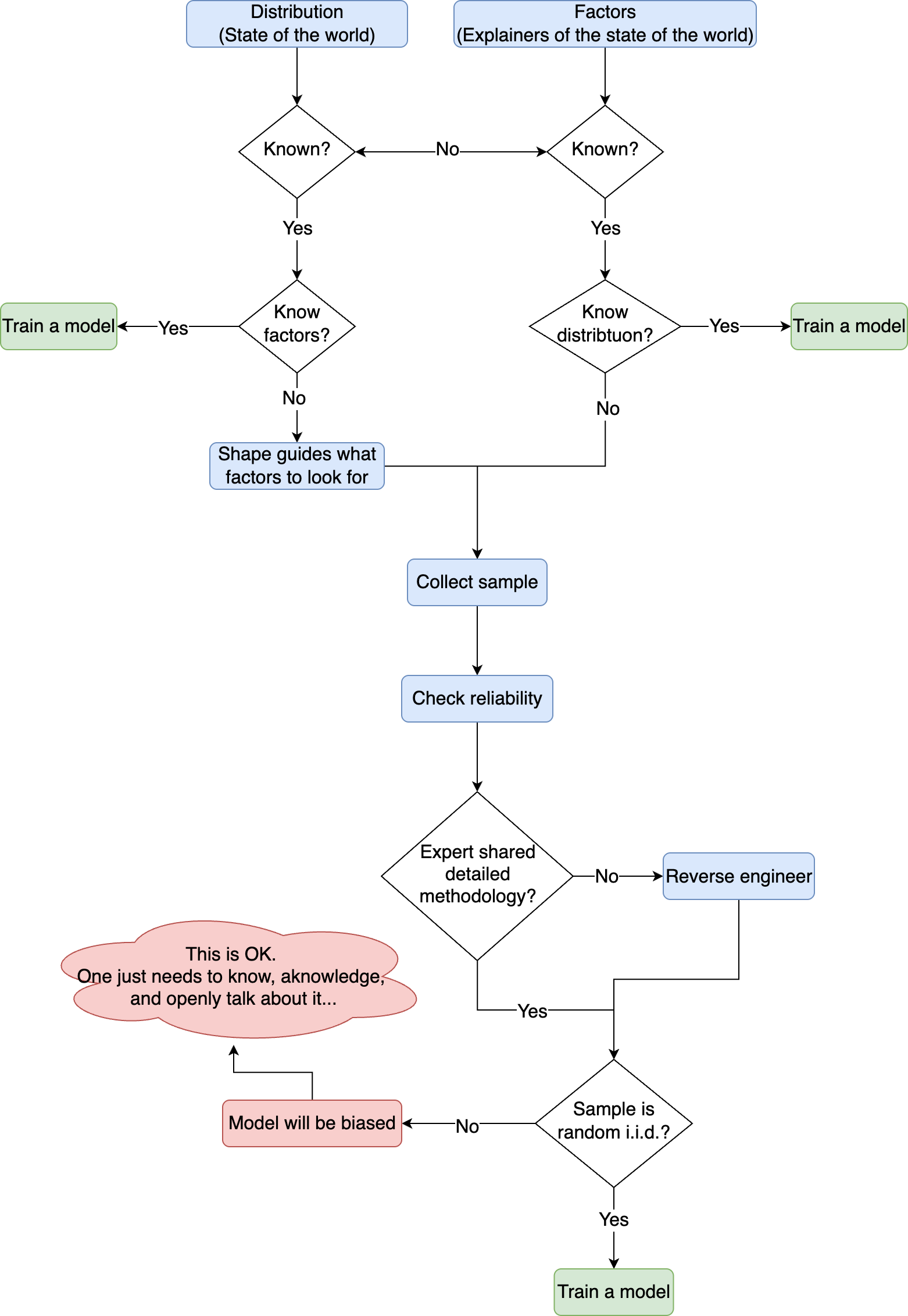

The word “distribution” is a truly monumental keyword. And since I have made it a central lighthouse to the turmoiling sea of my thinking, it has been doing wonders in guiding me!

When I ask:

“how to predict aqueous solubility?”

I am implicitly asking:

1. What is the state of the world for aqueous solubility (i.e., distribution)?
2. What are the factors that could be leading to this state of the world?
3. What are methods to help me map from these factors to this state of the world?

And each question includes a list of actions that are needed to answer it.

In this post, I can only touch on the first question. So, let’s start with it:

What is the state of the world for aqueous solubility (i.e., distribution)?

Now, I can approach this question from two sides:

1. I know the distribution shape.
2. I know how some factors interact to give me the aqueous solubility of a molecule.

If I know the distribution shape, this helps me identify where to look. Because each distribution shape has a reason to emerge in the way it emerges.

And if I know how different factors interact together to produce an outcome, I can anticipate the shape of a distribution. Because a distribution emerges from the ways these factors interact.

Let’s make this clear with some examples.

The normal (Gaussian) distribution

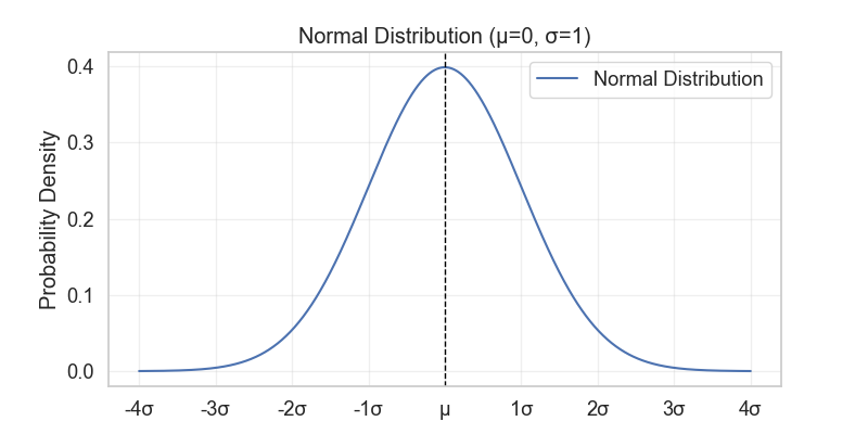
If something follows a normal distribution (Figure 1), then this thing is a result of multiple independent factors that “add” together to give rise to it (the reverse definition of the Central Limit Theorem (CLT) that was discussed in this post!).

For example, for aqueous solubility, we can think that many factors such as molecular weight, polarity, electronegativity, structural complexity, etc., are all factors that affect the aqueous solubility of a molecule. If all these factors are independent, and each one contributes a little bit to the property, then the aqueous solubility of all molecules will follow a normal distribution.

The other example from the last post on distributions was the female population height. We know that it follows a normal distribution, and this is because it’s the interaction of many independent factors like genes, nutrition, geography, etc. (are they really independent 🤔? That may be a philosophical question for later!).

So, if I know the distribution shape, then I already have a base for where to look next. And in the case of a normal distribution, it’s to look for independent factors that collectively will explain the distribution.

This can also be approached the other way around. If I know that something is the result of additive independent factors, then it will follow a normal distribution.

The bi(multi)modal distribution

The bi- or multimodal distribution is just a combination of two or more normal distributions (Figure 2, top left). When a distribution has more than one mode, this means that the question being asked is not as fine-grained (i.e., there is one or more factor that can separate the distribution into different group ranges).

Let’s recall the height distributions from the last post. If we ask “how tall people are?” we get this bimodal distribution (Figure 2, top right). That’s because there are two obvious groups here: kids and adults (Figure 2, bottom left).

Now, the factors contributing to the overall distribution of individuals’ height would probably be the same. If two siblings grew up in the same family, expressing the same gene, going through the same socioeconomic status, they will end up at the same height bin relative to their peers. The thing is, if their peers are adults, the bin will be at the higher end of the scale than if they were kids!

So, the only thing a bi(multi)modal distribution says is that there is a factor that is shifting the effect of all other factors to a different range. In the height example, it was the age!

Another thing to notice is that, while the kids and adults distributions look Gaussian, they actually consist of two groups each as well: females and males (Figure 2, bottom right). This tells us that there is a factor that, when combined with the age factor, makes another difference in height range, and this factor is the Y chromosome!

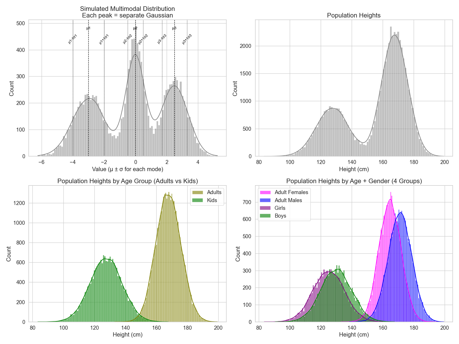
So, when something shows more than one mode, this usually nudges us to look for subgroups in the distribution. And if we know our question well enough, we can catch when something looks Gaussian, but it’s actually a sneaky multimodal!

An example of a multimodal distribution that can arise for aqueous solubility would be the different subtypes like kinetic and apparent solubility.

Now, kinetic solubility is a quick and dirty approach where a diluted compound is being tested for the first hint of precipitation. This setup is usually used as a quick diagnostic for filtering compounds rather than a final measurement ready to be taken in established protocols.
Apparent solubility is a long and exhaustive process of making sure that the crystal form of a compound is at equilibrium with the solution after precipitation (i.e., not going back to the solid state).

Just by pure definition of the two groups, I would assume the kinetic solubility to give exaggerated values compared to the apparent solubility. Therefore, if one mixes kinetic and apparent solubility values, one would end up with a bimodal distribution.

The lognormal distribution

The lognormal distribution is a cousin to the normal distribution, hence sharing the same last name (hehe)!

While a normal distribution is the result of additive independent factors, lognormal is the result of multiplicative factors. In more comprehensible English, the distribution emerges because there are factors compounding together and exaggerating the effect with each added factor.

An example is the income distribution. Now, one starts with a base salary, but then they keep getting promoted, and so, their salary increases by the percentage they got promoted with. So, the distribution of people’s income will keep jumping by the multiplication of the salary and promotions (Figure 3).

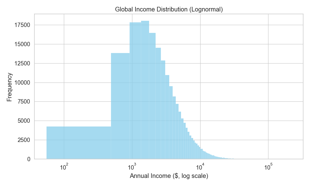
Aqueous solubility actually belongs to this category because, as physical chemistry suggests, it’s the result of multiplicative factors (lattice-free energy, hydration, conformation, ionization state, etc.).

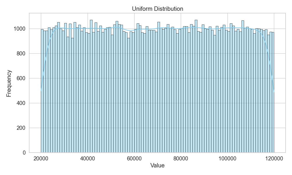
The uniform distribution

The uniform distribution is the “maximum entropy” distribution (i.e., random). It’s when there is no clue to decide whether something is more likely to happen than another (Figure 4). And if something is truly uniform, then there is no way to find factors that would lead to the distribution shape. This is the distribution where logic breaks and causality is no longer invited!

The uniform distribution is also the beginning state when asking a question that one has no idea how to answer. One assumes that everything is equally likely (i.e., the null hypothesis) and then goes on to uncover factors preferring a single outcome to another.

And it’s then when the uniform distribution starts shifting into any of the other distributions.

So, when one starts a question with zero intuitions or the ability to assume something (maximum ignorance), one is essentially assuming a uniform distribution!

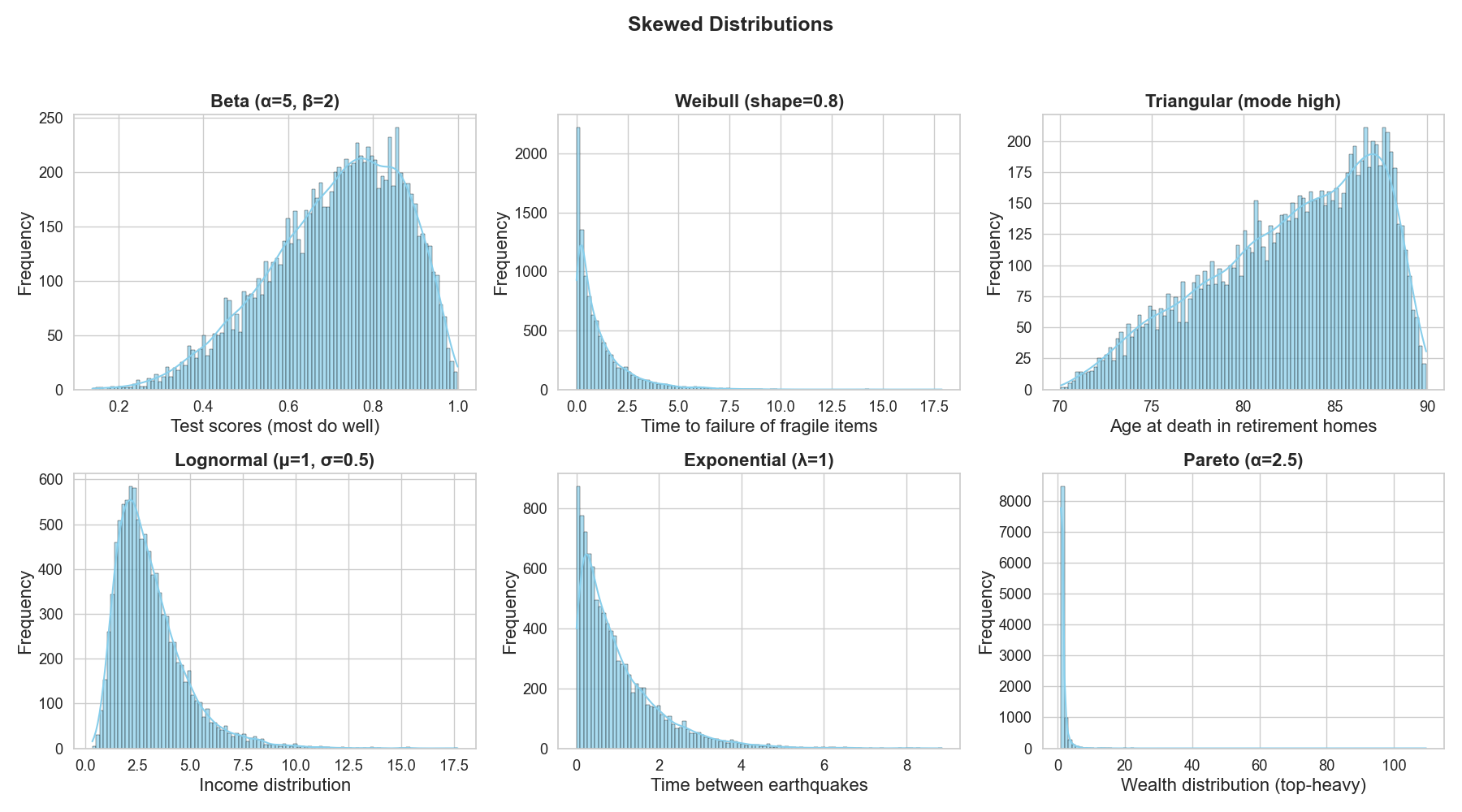
Skewed distributions

Skewed distributions is not the name of a certain distribution shape, but rather a description for a variety of shapes that are “asymmetric”! (Figure 5)

For example, the Gaussian and uniform distributions are symmetric because they look the same on each side of the middle of the distribution. A lognormal distribution is skewed because observations are piled on one side more than the other and then drags a long tail towards the edge.

The more skewed a distribution is, the more it becomes clear that the system is favoring certain outcomes or behaving in a very specific mechanism.

Take test scores as an example (Figure 5 top left). For one student, the number of right answers out of many questions follows a binomial pattern (only two outcomes, either correct or false). But if we look at the fraction of correct answers across the whole class, those proportions fall between 0 and 1 and can be described by a Beta distribution. The binomial handles one student’s successes and failures; the Beta smooths out the distribution of proportions across everyone.

So, it feels like if someone knows their problem well, they can pick the matching skewed distribution to describe it in general. Or, if someone lands the matching skewed distribution, they will know how to describe their problem accurately.

Giving a distribution to a model (The supervised learning version)

Now, if I know a distribution, I need to give it to a model alongside the factors contributing to it as best as my knowledge so far. Then, the task of the model is to tell me exactly how each factor contributes to this distribution.

Let’s take the height example: we say that it follows a normal distribution for females, and we suspect that factors like genes, nutrition, geography, and socioeconomic conditions are the main culprits.

Then, we give the model a list of females’ heights with their corresponding information, and the model figures out how much each factor contributes to the height of each individual approximately.

Now, for the model to approximate the true effect of each factor, the model needs to see “enough” examples to pick up on the nuances between the factors and the distribution. But…

How much is “enough”?

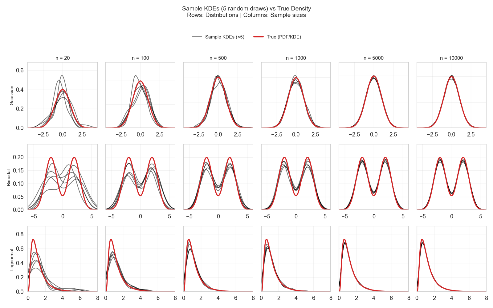
The traditional answer, as we have seen in the last posts, is “as large as possible.” But actually, this “large” is different for each distribution. For one distribution, a few hundred examples can approximate it very well, and for another, thousands of examples would be needed. The main culprit is the distribution’s simplicity! (Figure 6)

A small sized random sampling of a distribution gives an honest representation of its spread (i.e., variance \(σ^2\)), as seen by all the different random draws in the examples in Figure 6 (first column). And this is the exact reason why approximating the variance of a distribution does not require CLT, but simply knowing the variance of a single sample (this is what was done in this post!).

So, a distribution like Gaussian, which has variance as one of its two parameters, is already halfway there just from a single small sample (e.g., only 20 observations). The other thing needed is estimating the mean (µ), and this is the sole task of the observations collected from a normal distribution. That’s why after a few hundred observations, it becomes quite easy to know where this µ will converge (Figure 6, top row).

A bimodal or lognormal, on the other hand, has more nuance to it. For bimodal, one needs to estimate two variances and two means, while for lognormal one needs to estimate the variance, mean, and the multiplication mechanism. So, with each parameter needed to be estimated in a distribution, the more observations will need to be collected to cover enough examples.

In Figure 6, a few hundred observations were only good to assume which family the distribution would fall into (bimodal or lognormal). However, there were still visible uncertainties in landing the troughs and dips of the distribution.

In a distribution like Gaussian, one is dealing with a single uncertainty (µ), but with other distributions, one is dealing with more uncertainty.

Remember the random i.i.d.

Remember that this sampling needs to be random and respect the independent and identically distributed condition. By recalling this post, the identical distribution is straightforward once we have identified the question clearly.

If one is trying to represent the distribution of adult females, then one should not include examples from kids or adult males. This is how to ensure identical distribution.

One can still include the distributions of other groups if they are interested in the population height without fine-grained grouping. However, one needs to make sure that the model sees enough information to help it distinguish the different groups. Otherwise, the model can end up learning spurious (i.e., weird) relationships!

The random and independent conditions can be tricky here. One needs to make sure they are not introducing any bias while drawing the sample. For example, if one draws a sample for the female height distribution, but gets it only for one country, two things happen:

1. Violating randomness: All the data points will come from the same place, and the model will falsely think that geography plays no role in this distribution.
2. Violating independence: All heights will be within a specific range of the distribution because we know that geography affects height.

The problem with bias is that it relies on knowing what factors we suspect are important for a distribution!

For example, before one suspects that geography affects height, drawing a sample from a single country wouldn’t have posed a bias problem. But now, because we know it affects the distribution, we know that not paying attention to it will bias the sample (did you spot the circular reasoning here?).

So, until one has a perfect model of predicting an outcome from specific factors (i.e., causal relationships), one cannot really know how biased their sample is until the new piece of the puzzle gets resolved!

The only bias one can detect is bias given the factors known so far.

A working example of aqueous solubility — How to judge a sample quality?

Now, let’s start thinking through the logic of our model that is trying to predict aqueous solubility and check the distribution we are giving it.

We recall the figure of different dataset distributions shown again in Figure 7. We already mentioned that the AstraZeneca (AZ)¹ and BioGen² subsets are well-defined measurements because they reference the experimental setup directly (check this notebook).

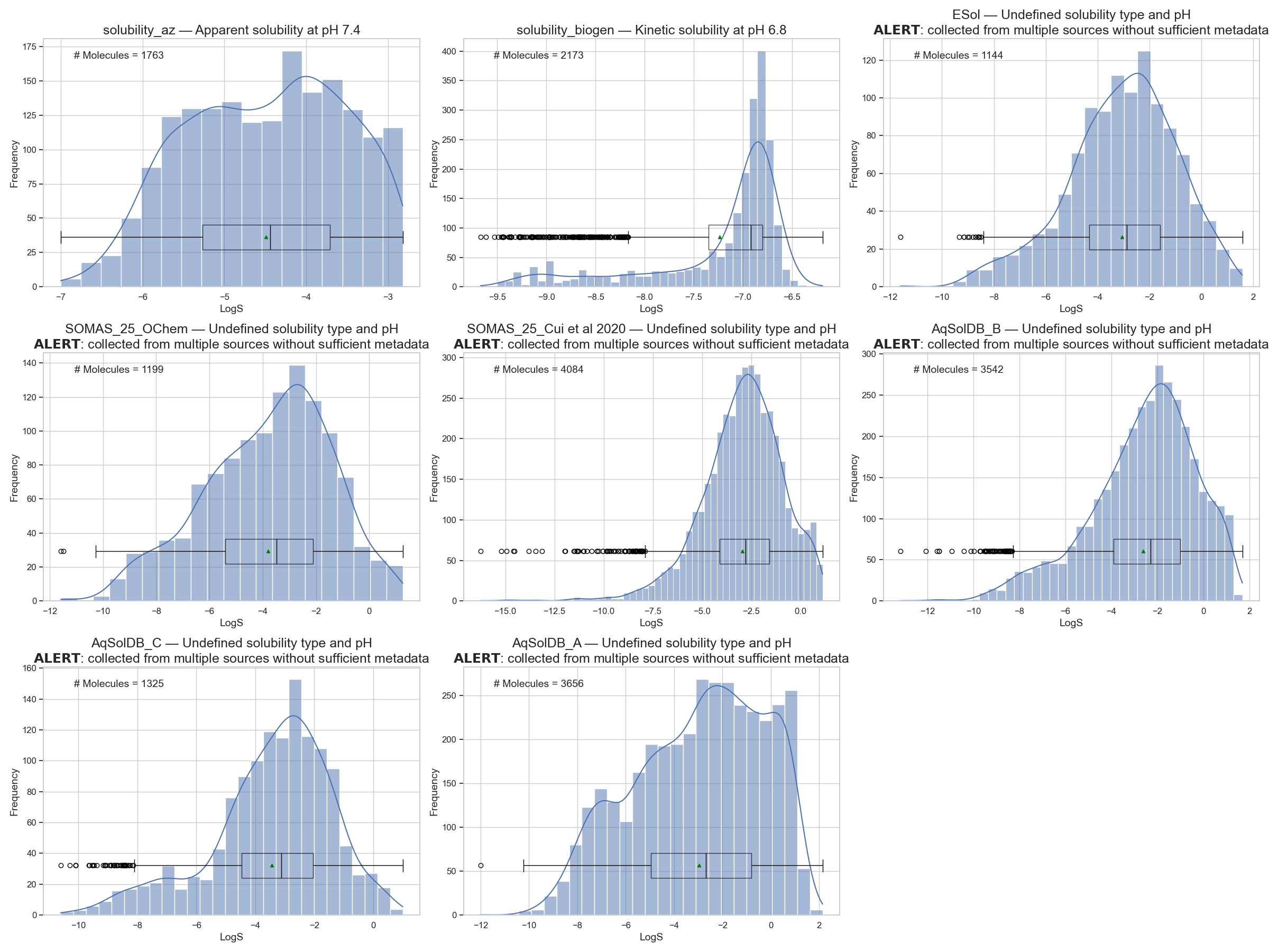
A database like AqSolDB³, while being a great feat in sanitizing molecules to SMILES and attempting statistical consistency for the same molecule, they missed the distinction of solubility types as explained by Llompart et al. ⁴.

Just by skimming the dataset curation in the AqSolDB methodology section, they mention that: they collected molecules from database A by filtering with the filters “experimental studies” and “water solubility.” This resulted in molecules with varying pH and temperature, which they further filtered to 25±5°C.
There is no further mention of filtering by pH, which is known to be a major factor influencing a molecule’s solubility (i.e., the same molecule can have different solubility values under different pH, and all values will be correct!).

In their description of dataset B, they mention that the molecules were in both liquid and crystalline forms. According to my limited knowledge of solubility, I would assume that this corresponds to kinetic vs. apparent solubility. And again, the same molecule would give different solubility values for each setup, and both values would be correct!

The way AqSolDB was curated was by merging databases, identifying duplicated molecules across the different sources, and then trying to set a statistically reliable value for each molecule when multiple values exist.
However, I don’t see anywhere in the manuscript where they acknowledge that these differences could be due to justified and important experimental measures, rather than inconsistencies requiring an aggregation scheme!

So, just by a few moments of pondering on the origin of the AqSolDB distribution, I can already conclude with some confidence that it violates the “independently distributed” condition for constructing a distribution.
Whatever is being represented in this distribution will be a mixture of distributions that have been further smudged by aggregation of the individual values.

So, my verdict on this dataset will be: Do not use unless one wants to confuse their model!

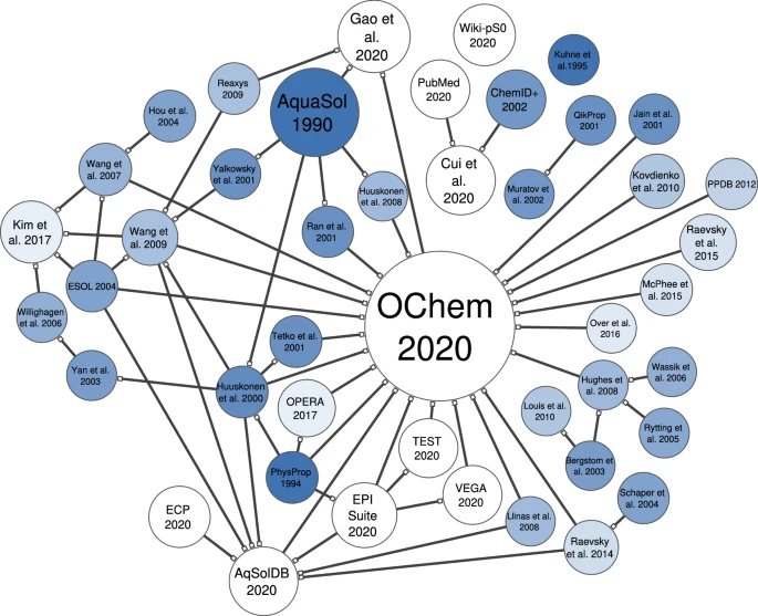
Now, unfortunately, many other databases have done a similar thing of aggregating datasets into a single big one. Yet they remained short in explaining the experimental origin of each molecule to understand which condition gave rise to each value (check the connection map in Figure 8 made by Llompart et al. for the different aqueous solubility datasets in the literature).

So, unless one goes back and double-checks the origins of these distributions, one needs to be careful not to feed their model with these datasets.

Even if the model learns something, it might be for the wrong reasons!

So, this leaves us with the AZ and BioGen datasets as possibly reliable distributions.

I will start by looking deeper into the AZ dataset to see the questions I will need to ask to make sure that I am feeding my model reliable distributions… and how to answer them!

The AstraZeneca sample

Now, the AZ sample is only 1763 molecules. So, it constitutes a sample rather than a true distribution.

And since this is a sample, I want to know how reliable this sample is! To know this, I would like to know how this sample was generated to answer the following questions:

1. Is this a randomly selected sample (i.e., is it a representative sample of the apparent solubility distribution)?
2. Is the data identically distributed?
3. Is the data independent?

So, I will need to go back to the methodology section of the dataset and see what the chemist shared with us.

Unfortunately, this dataset is only available as an entry in ChEMBL, and all the info available out there is shown in the below quotation — which is not much at all!

“ASTRAZENECA: Solubility in pH7.4 buffer using solid starting material using the method described in J. Assoc. Lab. Autom. 2011, 16, 276-284. Experimental range 0.10 to 1500 uM”

But at least I know now that it is measured at pH 7.4, and by checking the reference they used, it’s an apparent solubility measure.

This tells me that this dataset passes the “identically distributed” check.

Since the chemist left me hanging, the other things I need to know will have to be reverse-engineered from my inspection of the sample to the best of my abilities.

So, let’s start with the “random” check!

Is this a random, and therefore, representative sample?

One can approach this question from two different angles: statistically and chemically.

Statistically, I will need to:

1. Have an assumption about what the distribution would look like.
2. Consider what a random sample of this distribution looks like on average.
3. Ask: what is the probability that this sample is a random sample of this distribution?

So, what is our assumption on the apparent solubility distribution?

The answer will be half-fictional due to my limited experimental knowledge, but I will continue with it just to carry on an example and show logic rather than true answers.

A chemist is more than welcome to help me make this example real-life!

So, from the different distributions of aqueous solubility in Figure 7, while not all datasets are reliable, they at least show me that the range of the distribution is roughly between -12 and 2 LogS.

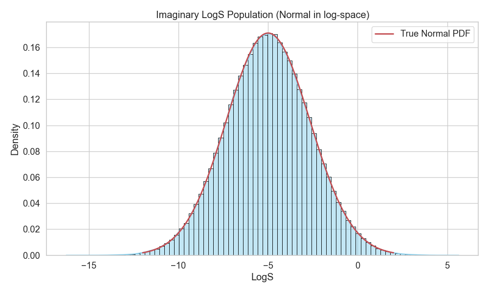
We already assumed above that aqueous solubility will probably follow a lognormal distribution because it is the result of multiplicative factors. So, we will assume that the true distribution is a lognormal between -12 and 2 LogS.

Since we are using LogS units and not the raw Mole/Liter, this will already make the distribution look Gaussian (i.e., lognormal distributions show up as Gaussian on a log scale, hence, the “normal” part of the name).

With this, we have our assumption of what the true distribution would look like (Figure 9).

Now, let’s see what random samples would look like by drawing them from the imaginary distribution.

First, we need to notice that the AZ sample ranges between -7.5 and -3. So, it is already biased within the distribution to this range.

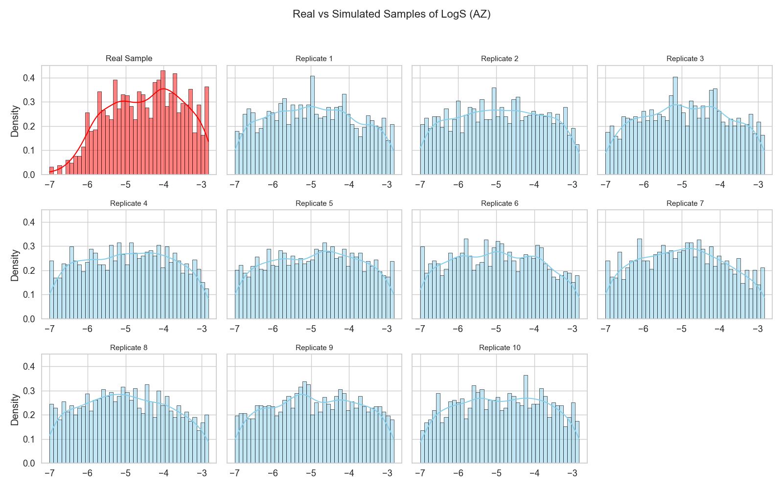
When I want to check what a random sample looks like to compare against my AZ sample, I need to compare it to random samples that will be drawn from this specific range with this specific size (Figure 10).

The randomly drawn samples in Figure 10 show more or less a uniform distribution, and if one squints their eyes, they can see that AZ was trying so hard to follow a uniform distribution as well.

However, if one were to use a statistical significance test, the p-value would probably say that the AZ distribution is different from the replicas, and therefore, it would be judged as “not random.”

However, everything needs to be put in context and not just measured against some fixed numbers or equations.

Let’s stop for a moment and ponder what this AZ sample means.

Firstly, a chemist doesn’t know in advance what the solubility of a molecule would be.

Secondly, it looks like the chemists were trying to restrict their analysis to a specific (and narrow) range of the distribution.

Now, this looks like a game of shooting darts blindfolded. The fact that the chemists managed to make the sample that close to the random replicas in Figure 10 is already a great feat!

One does not need to consult a statistical test in this case to determine if the sample was randomly drawn to the best of human abilities!

So, my verdict on this sample is: it looks statistically randomly sampled to me (i.e., representative).

A chemical inspection of “random”

A chemical inspection of the “random” check would need to go in the direction of molecular diversity.

Are the molecules diverse enough, or have they been selected only from a specific region of the distribution?

This part is trickier than the statistical part, and it requires more chemical knowledge. But one thing I can use is the concept of chemical series.

Chemical series occur when molecules share the same backbone structure, but differ by extensions to this backbone (Figure 11).

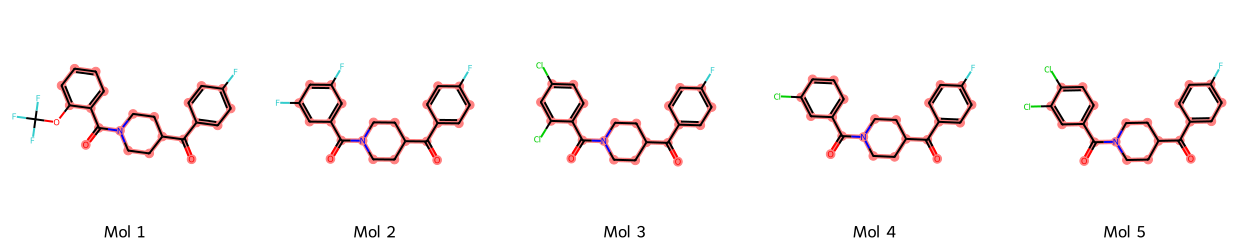
This means that while many molecules can give different solubility values — giving the feeling of statistical random sampling — they might be chemically clustered, therefore violating chemical random sampling.

Now, to determine whether two molecules share the same chemical family, one can strip two molecules of any branches and additions, keeping only the backbone, and see if they match.

And this is exactly what an algorithm called Murcko scaffold does. It extracts the scaffold (i.e., backbone) of each molecule, and then one can see whether some scaffolds are more frequent than others and by how much.

Running the algorithm on the AZ molecules showed that the sample has ~1K unique scaffolds. This means that ~60% of the molecules have their own scaffold that is different from the others!

Figure 12 shows the 50 most frequent scaffolds in the AZ sample. The most interesting thing to notice is that the most frequent scaffold is found in fewer than 2% of the molecules.

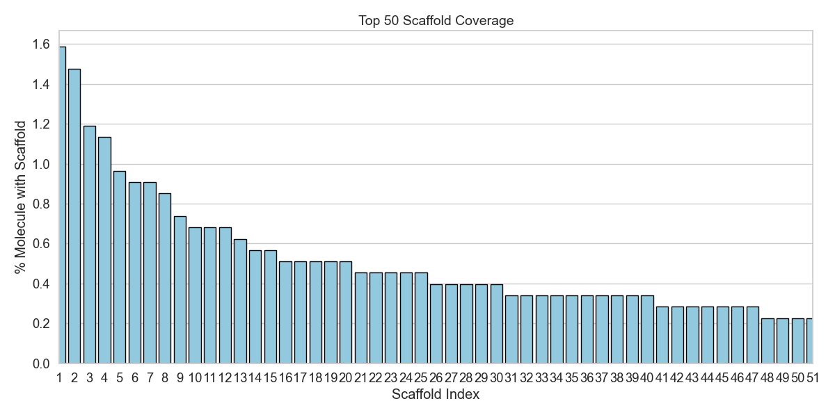
So, this simple chemical inspection further emphasizes the statistical verdict: the sample is indeed randomly drawn, and therefore, representative of a real apparent solubility distribution for the range it was restricted to!

With these analyses, I can conclude that the AZ sample is identically distributed and representative of the problem I am trying to solve. This is already a great reliability verdict.

The third question remaining for this section is: Is the data independent?

What this question asks is basically: are there molecules that are too related, in the sense that knowing the solubility of one molecule makes me know the solubility of another one?

And this question cannot be answered by eyeballing the solubility values. It can only be answered within the realm of the factors affecting the distribution, as well as information theory.

And this is a feat that is gonna take too long on its own!

So, for now, and after this monstrous blog, one takes a reeaally long and deep break before coming back to tackle more questions!