In the last two posts, I was trying to answer a question but found that it only became entangled with the limitations of reality. To know how good a model is, I need to land on the true distribution of its performance—to see what is common and what is rare. However, this requires a large number of i.i.d. samples, which unfortunately are not easy to find in our field.

The road from here is no longer about finding the answer, but about making a truce with our messy world.

This post is also accompanied by a notebook to reproduce the figures and explore the concepts shown below.

TL;DR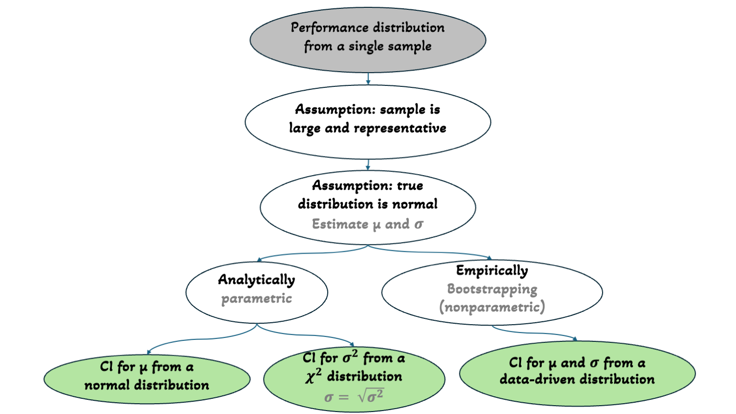

Check this post for an update to the logic mentioned here.

I would like to start this post with the following statement:

Once I understood that my model is only faithfully represented through a distribution that is not easy to pin down, I realized that the next step is to turn to uncertainty rhetoric that would say:
“Given this dataset, …”
“Under the current limitations, …”
“My model can do … but not …”

In this post, I will be discussing the situation where one has a small dataset of a couple of thousand molecules to train a model that predicts aqueous solubility.

Every approach to be discussed in this and the following posts will no longer answer “how good will my model be on new molecule(s)”, but instead one or more of these questions:

• How well did my model learn this dataset?
• How robust is it on this dataset?
• Which predictions should I trust, and which not?
• When will the model break?
• Do the predictions make sense?

I believe that the battle to answer the big question is lost for the time being under the current conditions. The best one can do is make a truce, lick wounds, take a deep breath, look around, and figure out how to make lemonade 🍋…

The lemonade stand

So, let’s start making this lemonade. I already stated that all the ingredients I have access to are small datasets of a few thousand molecules. Let’s step out of simulation land and start doing real-life modeling and error distributions.

Let’s revisit the aqueous solubility datasets’ distribution I showed in the last two posts (Figure 1):

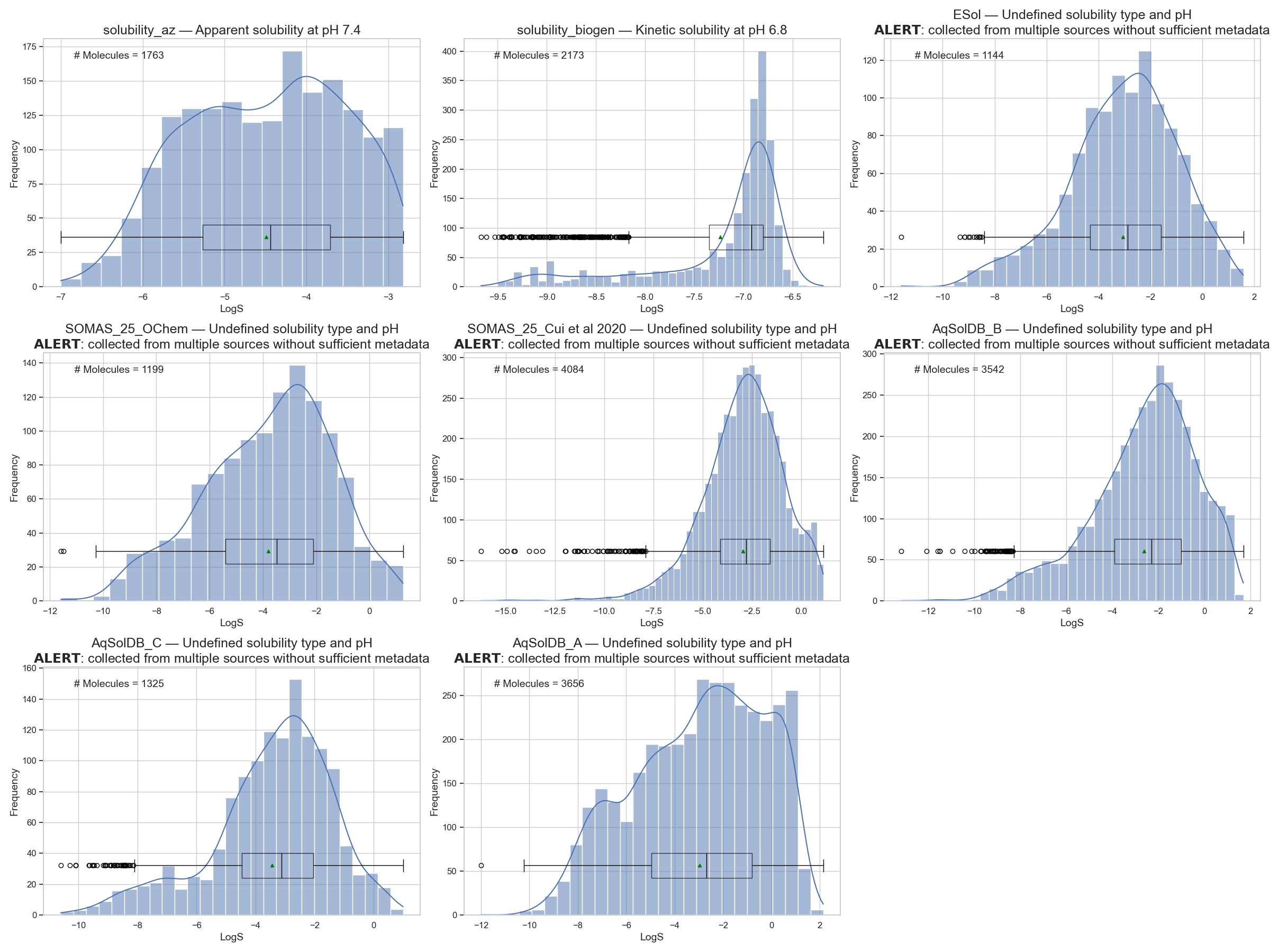
I will pick one of these datasets to model—preferably one without an “ALERT” header. I will go with the dataset from AstraZeneca that measures apparent solubility at pH 7.4 for 1763 molecules. But any other dataset can be used in the accompanying notebook.

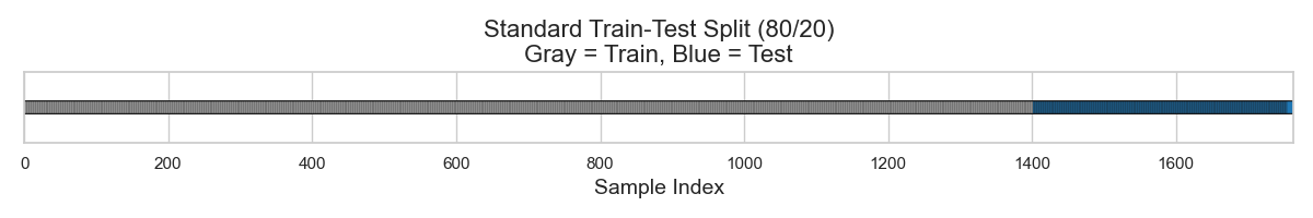
As recalled from part 1, the simplest starting point is to split this small dataset into a train-test split, say 80:20. Doing so results in 1410 molecules for training and 353 for testing (Figure 2).

I will use RDKit descriptors to represent each molecule. These descriptors range from physical chemistry (e.g., molecular weight, polarity, electronegativity) to structural information (e.g., ring counts, atom types, branching patterns). Each molecule is thus converted into a numeric vector, where each number corresponds to one of these descriptors.

I will then throw a random forest (RF) model at my training data. The hope is that the RF model will learn how these descriptors interact to estimate the most likely solubility value for a molecule.

Let’s say my model learned that when a molecule has x hydrogen bond donors, AND < y molecular weight, AND a > z polar surface area, it is more likely to have a solubility around -2 LogS.

So, I train my RF model on the 1410 molecules, hoping it captures such meaningful interactions between these descriptors. I then test it on the 353 molecules and get the residual distribution shown in Figure 3.

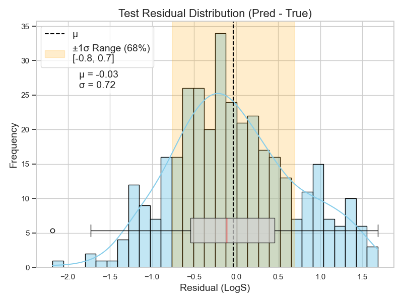
Now, this plot is telling me quite a lot. It shows that the average error of my model on these 353 molecules is almost zero. However, the standard deviation shows that 68% of the errors fall between -0.8 and 0.7 LogS.

The distribution shape also shows that my model makes more positive errors. The right side of the distribution is heavier than the left. Notice, too, how the mean (dashed line) is pulled to the right of the median (red line) in the boxplot.

This means that my model tends to predict higher values than the actual ones. For example, if a molecule’s solubility is -6 LogS (i.e., 1 µM), my model was more likely to predict something like -5.8 LogS (i.e., 1.6 µM).

But let’s not forget: this is the anecdotal case of my model’s performance on these 353 molecules. The distribution’s mean, standard deviation, and shape can differ slightly—or significantly—if the model were tested on a different 353 molecules.

So, what I need to do is to inject uncertainty into my speech about my model. I want to have a feeling—or at least a clue—about how off these predictions might be given my current inputs.

Estimating my distribution parameters

Now, let’s revisit the assumptions about my model performance.

In the best-case scenario where my data, my representation, and my model are all perfectly working together, the model should be able to learn everything there is to learn about the data using my representation.

The remaining unlearned patterns would be just noise. And this noise is expected to follow a normal distribution with mean zero.

A normal distribution with mean zero means that the majority of my errors will be within one standard deviation from the mean (i.e., my predictions are mostly accurate).

Therefore, if I manage to estimate the mean and standard deviation of my model’s performance distribution, I can construct it easily.

In the last post, I already discussed how the law of large numbers (LLN) and the central limit theorem (CLT) are helpful when estimating a distribution’s mean.

However, I also noted that many i.i.d. samples are needed to construct a distribution of the means, and then compute a confidence interval (CI) that bounds the true mean.

But in the current case, I only have access to one sample of 353 molecules.

So, how can I apply CLT? There are two ways to do so…

1. The leap of faith — analytical statistics (parametric)

The distribution of means is itself a distribution that we want to approximate in order to estimate the CI of interest. Statistics has a way to construct information about a true distribution from a single sample, under two assumptions:

• The sample is large enough
• The sample is representative

When using this leap of faith approach, I assume that these two assumptions are met, and then calculating the CI follows these steps:

1. Estimate the standard deviation of the means distribution using the sample standard deviation \(s\) and sample size \(n\):

   \[\text{standard error of means (SEM)} = \frac{s}{\sqrt{n}}\]

2. Estimate the CI of interest using the sample mean (\(\bar{x}\)) and the critical value \(t^*\) from the t-table for the corresponding % of interest:

   \[\text{CI} = \bar{x} \pm t^* \cdot \text{SEM}\]

Since I already know my sample mean and standard deviation (-0.03 ± 0.72), and for 95% CI, the \(t^* = 1.96\) (from a predefined table), then:

And the range that bounds my true mean turns out to be:

With this, I have an idea of the upper and lower bound of my true mean, which is one pillar for constructing a normal distribution.

The second pillar is to know the true standard deviation…

Estimating standard deviation

The reason I can estimate a CI for the true mean from a sample mean is that probability and the LLN guarantee that sample means converge to the true mean. The CLT then guarantees that this convergence follows a normal distribution.

The other value defining a distribution—that is also guaranteed to be approximated from a sample—is the variance (\(σ^2\)). However, CLT is not needed to tell us the shape of this approximation.

Probability theory states that the distribution of variance follows a chi-squared (\(\chi^2\)) distribution (Figure 4).

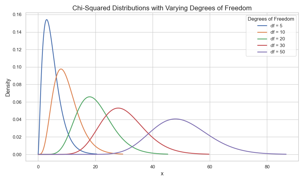
And just as there is a formula and a table for estimating CIs of a normal distribution, there is one for the \(\chi^2\) as well.

Using this predefined information, I find that the 95% CI for estimating my model’s true σ (taking the square root of \(σ^2\)) is 0.67 and 0.78 (check the notebook for details).

2. The data-driven leap of faith — Bootstrapping (non-parametric)

Building on the same two assumptions (i.e., my test set is large and representative). The main idea is to sample K samples of size N from the residuals distribution of the test set.

This resampling selects points from the distribution with replacement (i.e., a single residual value can appear multiple times in the same sample)¹.

This “with replacement” feature ensures that each bootstrapped sample will form a slightly different distribution, leading to variation in the means distribution.

Once I have my K samples, I plot the mean of each sample and calculate the CI empirically by checking the corresponding percentiles on the means distribution (Figure 5).

For example, for 95% CI, I check the values on the tails where only 2.5% of the data are below and above, and this becomes my 95% CI range.

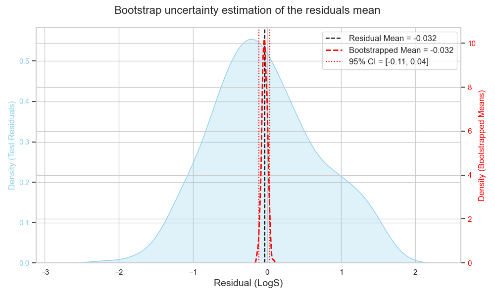
Here, the 95% CI is -0.11 and 0.04, which is quite close to what the first approach gave!

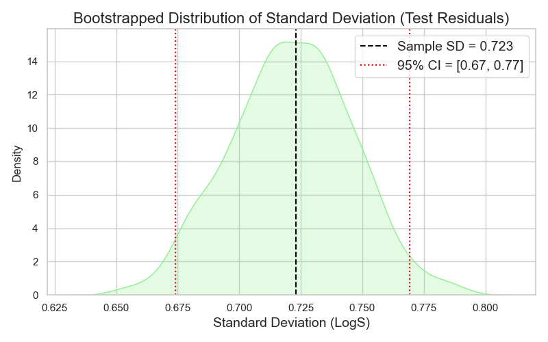
Estimating a range for my σ follows the same logic. I plot the distribution of the different samples’ standard deviations, and empirically select the 95% CI to represent my upper and lower bound, which turns out to be 0.67 and 0.77 (Figure 6).

This agreement between the analytical and empirical approaches for both µ and σ assures me that my assumptions about the underlying distributions of µ and σ were correct, and that my sample was representative enough.

The benefit of bootstrapping is that it does not require a predefined table of statistics like the t- or chi-tables (i.e., no distribution assumption).

However, to use bootstrapping effectively, one needs a sample large enough so that resampling with replacement does not produce overly similar samples. Usually, n > 10 is recommended, since the possible combinations of unique bootstrap samples at n = 10 are only about 9K.

Plotting my “true” distribution

Now that I have bounds for my µ and σ (from either the analytical or empirical approaches), I can start constructing an assumed normal distribution for my model’s performance.

Since I do not have a single value for µ or σ, but rather a range, I can think of constructing best- and worst-case distributions.

• The best case for the mean is µ = 0 (i.e., predicted = true).
• The worst case would be either bound of the CI range.
• The best case for σ is the lower bound (lower σ = more consistent predictions).
• The worst case for σ is the upper bound.

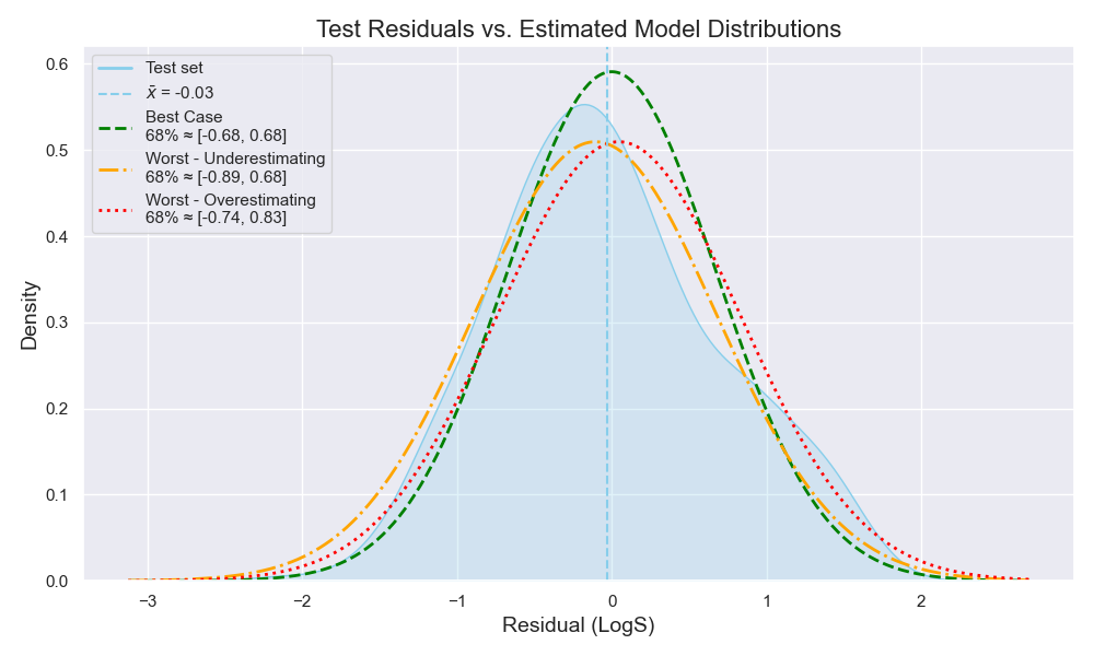
This means I can build three distributions -here, using the empirical CIs- (Figure 7):

1. Best case with µ = 0 and σ = 0.67
2. Worst case where the model underestimates the true value (µ = 0.04, σ = 0.77)
3. Worst case where the model overestimates the true value (µ = -0.11, σ = 0.77)

From these three distributions, I can go to my chemist and explain how my model would perform if all the stars aligned—or if they all collapsed.

And it is my chemist’s answer that should guide me on whether my representation and model are good enough to proceed…

Or whether I need to re-trace my steps and see which areas can be further improved.

Wrapping Up

Let’s summarize:

• With small datasets, the battle for the true distribution is often lost.
  • The goal shifts to making a truce and quantifying what can still be learned.
• One needs to identify their assumption on the true distribution, to identify which parameters to estimate and how
  • For a normal distribution, one needs to estimate µ and σ.
  • Estimation can be done analytically (with assumptions) or empirically (with relaxed assumptions).
• A single true distribution may not be the way, but rather, multiple distribution for the best and worst cases based on CIs.
• When one is limited in quantity, one needs to compensate with quality and rigor.

Final remark

The reason I am using leap of faith with the two approaches is that I am assuming my single sample of 353 molecules is reliable enough to hold the underlying assumptions.

It is usually very easy to forget or overlook assumptions. However, in every step along the road, loads of assumptions are being made. If one keeps forgetting about them, one only ends up surprised when things do not always work as expected.

To ensure that the assumptions stated here are met, one would need to:

1. Verify the test set reliability by a measure of chemical exploration and/or through consultation with a chemist to see if they would be satisfied with such a test set.
2. Find a way to test different test sets that are distinct from each other, and with persistent trends, one can assume that the model is robust against these assumptions.

If one does not have a solid chemistry background or a chemist to consult, then it is option two to the rescue.

And this will lead us into the cross-validation territory.

And I promise to bring something new with each blog post on this topic. 😉