In the last technical post, I talked about how to tell when one is in a state to start comparing models. I found that I needed to satisfy some conditions before concluding that my model is suitable for my data and representation. Now, assuming that I have such a suitable model and I want to compare it to other suitable models—or I found no such model, and I just want to see which of my suboptimal models is the least suboptimal—Is cross-validation the next logical step?

Short answer: Not as we use it today!

When I started my master’s thesis, my supervisor emphasized the importance of cross-validation to get a reliable basis for selecting a model’s hyperparameters. After a while in the thesis, we ended up selecting the “best” hyperparameters, and then tried to “compare” it to other models.

By this stage, I guess my brain kinda froze on using cross-validation in general, rather than for hyperparameter tuning only. So, I would end up with multiple performances for these different folds.

I guess my brain also said, “the more, the merrier”! I took the average of each fold’s performance, I represented it as a boxplot for each model, and I picked the model with the best-looking boxplot.

This approach felt intuitive to me (i.e., test a model on different folds and pick the model with the best overall performance)!

When I started my PhD in cheminformatics, this was basically the standard. People would perform cross-validation to test models on different folds and select the best model on these folds.

We even now have a great guideline paper by Ash et. al., 2024 that recommends which type of cross-validation to perform and which visualization and analysis to apply to it.

So, I basically had no reason to doubt my primary intuition.

However, I believe that now—with everything I have been exploring since I started working on this blog—I do!

This post is accompanied by a notebook to reproduce the figures and explore the concepts shown below.

TL;DR

But, before I attempt to answer whether cross-validation (CV) is suitable for models comparison, there are two things I need to define:

1. What do I mean by “models comparison”?
2. What is cross-validation?

What is “models comparison”?

I will stay faithful to the definitions I have been using all the way along this series. When I compare models, I compare their performance on unseen data.

In this setup:

• I have a dataset and a representation for this dataset.
• I select an algorithm to learn the relationships between the data and the representation.
• I test whatever the model has learned on a fresh sample of unseen data to see how good these learnings are for prediction.
• I collect the errors this model makes for each new data point.
• This collection helps in getting the distribution of this model’s performance (i.e., all the possible error behavior of this model on unseen data).

Now, when I think of “models comparison,” I am basically thinking of comparing these distributions of performance.

So, in this specific usage of the phrase “models comparison,” one:

• First estimates the performance distribution of a model.
• Then compares it to another distribution of another model.

The premise of this definition is that I have a dataset for training, and another dataset for testing. In real-life situations, this can be thought of prospectively as training on the data one has, then waiting for new data of interest to test the model on.

However, as shown in Figure 1, a clever approach is to mimic this real-life situation by splitting one’s existing data into train and test splits. This bypasses the need for waiting, and hopefully provides a faithful representation of what the model can do.

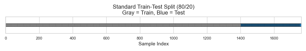
Now, what happened in Figure 1 is that I had a dataset of 1763 datapoints, and I arbitrarily chose to split it as 80% for training and 20% for testing. This gave me a set of 1410 datapoints for training my model and 353 datapoints for testing it.

My hope is that my 1410 training datapoints would:

1. Provide enough recognizable and informative patterns for my model to detect.
2. These patterns will be good enough to predict my test set.

The model will learn “something,” and the test set will reveal the error distribution of what this model has learned.

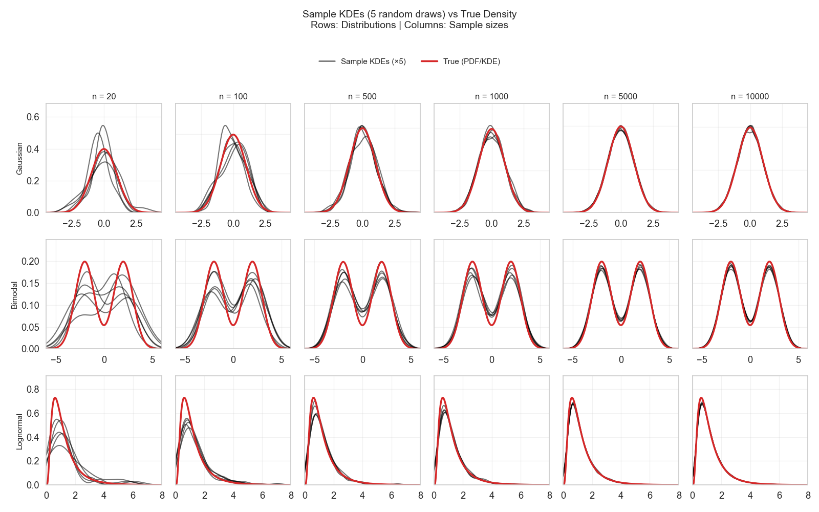
I was already lucky that my test set was as big as 353 datapoints. As shown in the recurring Figure 2, a sample of \(> 300\) datapoints is good enough to roughly estimate the shape and some of the parameters of different distributions.

So, with such a test set, if it is guaranteed to be i.i.d., I have a good approximation of my model’s possible error behavior on unseen data!

Yet this setup can evoke other contemplative questions like:

• Is 1410 datapoints enough to learn meaningful patterns that will generalize to unseen data?
• Are all models requiring the same amount of data to train well, or do some models need more data than others?

I will have to ignore these questions for now and remember one of the conclusions of the last technical post.

Maybe my setup is faulty, but I am trying to judge whether I extracted all that is there to extract, rather than judging whether I reached the nirvana…

What is cross-validation (CV)?

CV is a clever idea that stems from the same clever idea above. Instead of splitting the data one time, let’s do it K times!

Figure 3 visualizes this idea using 5-fold CV. In this figure, the data is segmented into equal folds (here, it’s 20% each). Then, each split provides different 80%–20% sets than the next one.

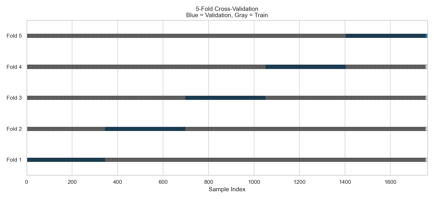
The model discussed above was trained on the first four folds (80%) and tested on the fifth fold (named Split 5 in Figure 3).

What happens to the other splits?

Well, the same model can be trained again, but each time, the train and test data are “slightly” different from the previous one.

By doing so, I will end up with five error samples for a given model.

OK!

But…

Why would I do this?

Why cross-validation (CV)?

The pre-packaged answer to this question is: to reduce test-set selection bias.

And, if this answer feels a bit gibberish—high five!—it did to me too!

So, let’s further explain it.

The premise behind this answer relies on the existence of multiple models. All models have been trained on the same train set, and tested on the same test set.

Now, if I want to select one of these models to be my best performer, one thing I can do is to select the model with the lowest error on the single test set I have.

But… the trap is, this model was better than the other models on this test set. Would it persistently be better than the others if tested on new test sets?

CV says, let’s test all models on different test sets and pick the one that will consistently perform better.

If a model persists across different folds, then this is surely a “superior” model.

Is persistent performance always good?

I have faced and combated the same exact question CV tries to answer in the past parts of this series! However, I was approaching it from the angle of estimating a single model’s true performance.

Analogously, the presumed goal of CV for model selection is to estimate the true best model.

When I tried to see the conditions needed for estimating the true performance of a single model, I realized it is either:

1. A large representative test set
2. Multiple small i.i.d. test sets

I then noticed that the words “large” and “small” are vague. So, I tried to understand what large and small mean in terms of distributions, sample size, and parameter estimation.

This was explained in detail in this post and where Figure 2 was first introduced.

After this post, I learned about the different shapes of distributions, the type and number of parameters needed to estimate a distribution, and how to judge “large vs small” for each distribution.

In the specific scenario of my 1763 datapoints, the test set of 20% was 353 datapoints.

When I trained multiple models in the last technical post, their error samples of this test set all hinted to a normal distribution (Figure 4).

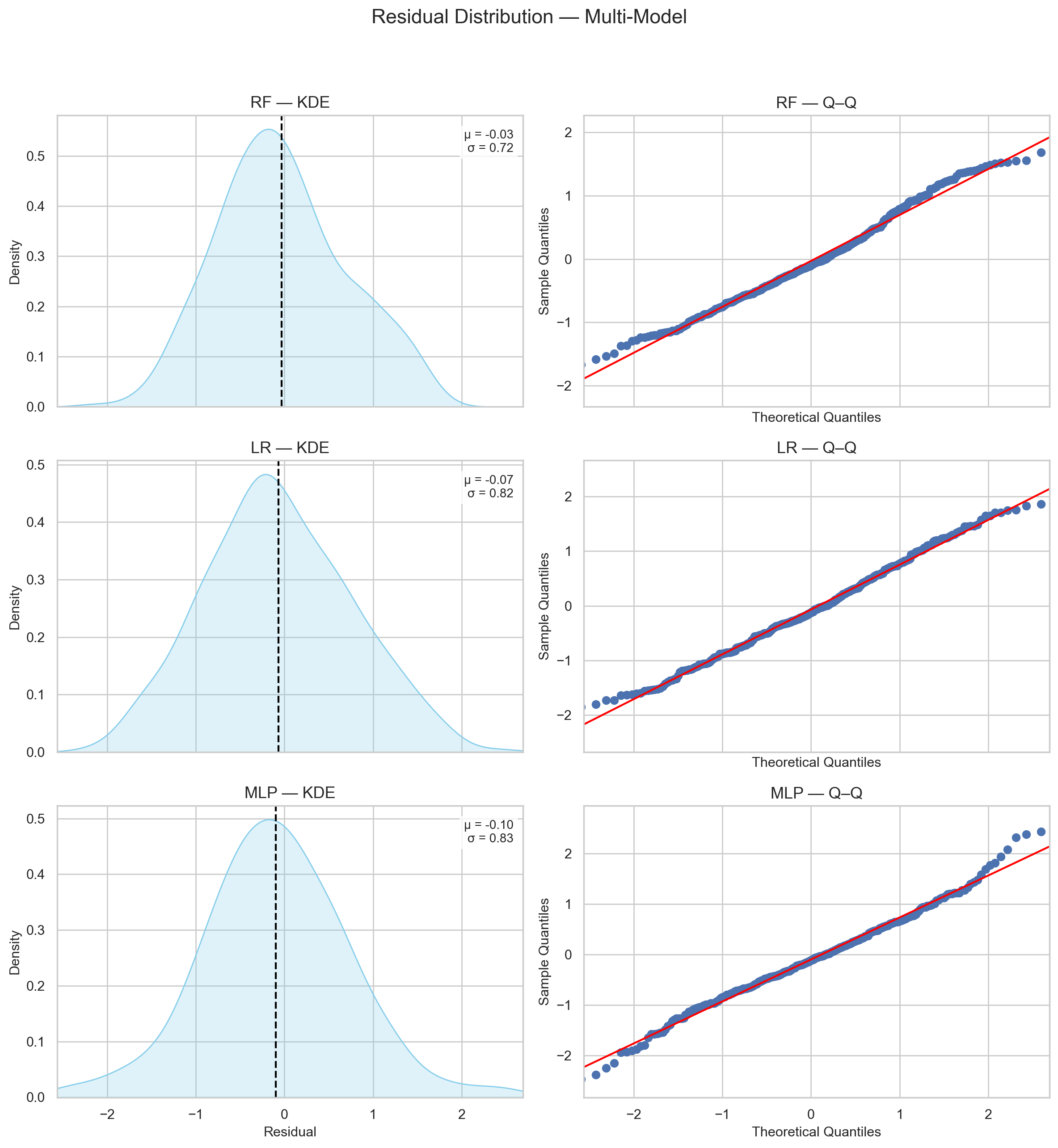
By consulting Figure 2, if I know for sure that my test set was random, representative, i.i.d, then I can easily estimate the true distribution of each model from their error sample with high confidence.

Therefore, deciding whether my single test set (a single sample) is enough to estimate my true distribution will vary based on two steps:

1. Recognizing how much data I need to estimate my distribution shape.
2. Identifying how much data I need to estimate the parameters of this distribution with high confidence.

Check this post for more details.

So, for this specific dataset of 1410 datapoints for training and 353 datapoints for testing, and an error distribution that points to normality, my test sample was sufficient to estimate my model’s true performance (assuming random, representative i.i.d.)

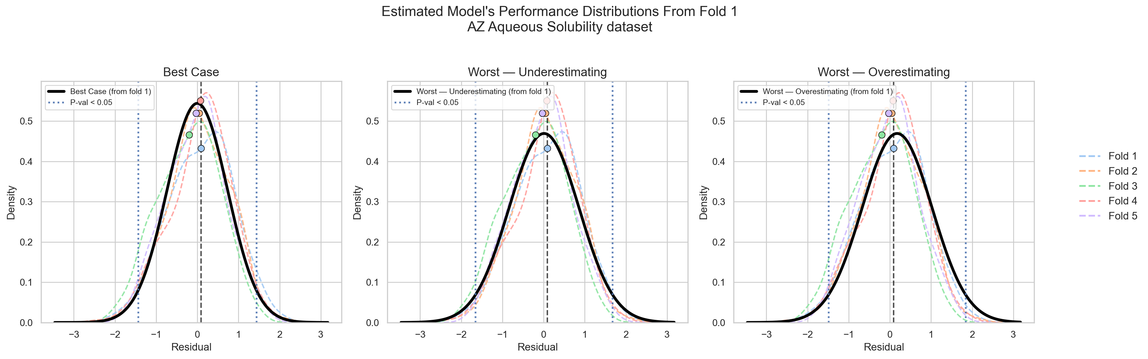
If someone gave me another test set of 353 datapoints, I have no reason to suspect that their errors will deviate significantly from the distribution I have already estimated from the first test set (check Figure 5).

If my first test set was random, representative, i.i.d., and large enough to estimate the true distribution, then any unseen data to come must fall into this distribution.

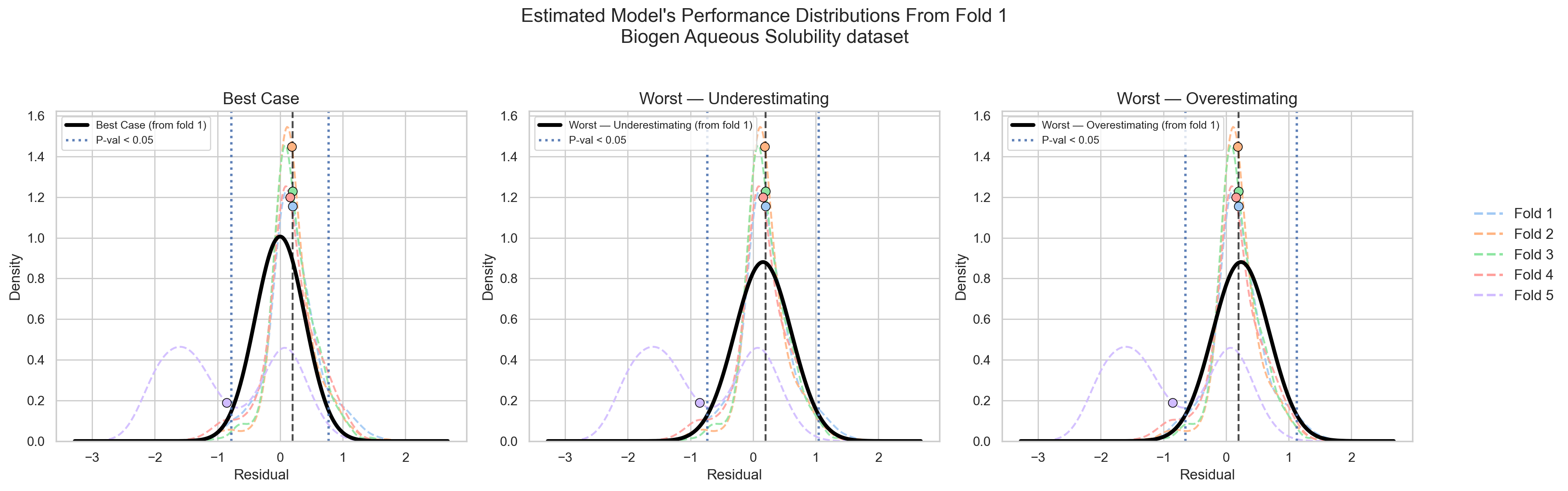
What to do if a new test set violated this expectation? (Check Figure 6)

Stop the analysis…

I do not think there is a point in moving forward in the analysis if one faced such a case.

This is a state of anomaly, and one needs to identify its source.

This can hint that either my old test set or my new test set were faulty. One of them probably violated the random, representative i.i.d. conditions.

If I ignore this alarm and move to model comparison and selection anyway, I will probably end up selecting a model that gave “better” values for the “wrong” reasons.

Because something was wrong in my data, but one model performed “better” nonetheless.

Did this model learn true signal or clever noise? Will it truly generalize to new unseen data?

The answer may be “a true signal,” and it may be “a clever noise.”

It can also be “clever noise that can generalize to unseen data”! (e.g., intrinsic measurement noise; an irrelevant signal in terms of chemistry, but relevant to prediction).

But it may never be clear until the incident gets investigated…

By extrapolating this logic to cross-validation as shown in Figure 3, each fold consists of 353 datapoints.

If all folds are random, representative i.i.d., then all of them should give me the same performance distribution (Figure 5).

If they did not, then I would assume that CV will not be giving me new information on my model’s performance, but rather, on my data itself! (Figure 6)

And if it was my data showing inconsistency, would it make sense to say that model A is better than model B?

The more logical question to me would be: What is it exactly that each model is learning? Which model to trust (if any)?

Understanding the cross-validation formalized by Stone in 1974!

The original concept of cross-validation has existed since the late 1960s. However, it was formalized as a data-driven decision-maker by Mervyn Stone in 1974.

His paper was named: “Cross-validatory Choice and Assessment of Statistical Predictions ”

I understand that Stone’s paper was quite a revolution for the time it appeared. He probably was the first person to formalize the predictive machine learning scheme we use today!

Before Stone’s formalization, inferential goals dominated statistical practice. A statistician would look at the data and figure out a function that would fit it.

The goal was not to generalize or to predict unseen data, but to find the function that would explain this data.

The scheme of that time would be analogous to model.fit() with minimal care for what model.predict() can actually offer.

Stone, in his cross-validation formalization, was the first to propose a formal way of running a prediction phase, then using the outcome of this prediction to select a function that would succeed at predicting this data!

Inference (i.e., finding the function that explains the problem) is no longer the holy grail in Stone’s scheme; it’s prediction.

Inference can happen as a byproduct. But… if it never happened, yet the function can predict correctly anyway, then hooray anyway.

The groundbreaking part of Stone’s work was giving birth to a formal scheme of data-driven predictive machine learning!

Instead of a statistician picking a function through inference, the data pick a function through prediction.

And Stone’s paper was to provide a robust framework to what this data-driven procedure would look like.

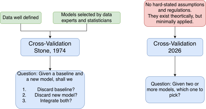
Stone’s CV vs. current CV

Current cross-validation for models comparison is performed as discussed at the beginning of this post. A person runs some model on different training-testing folds, then picks the model with the best-looking performance.

Best performance has been considered in terms of an evaluation metric like the mean absolute error (MAE), mean squared error (MSE), coefficient of determination (\(R^2\)), etc.

However, this was not the exact scheme that Stone proposed!

Stone envisioned cross-validation to be a process that guides one to answer two questions:

1. Does this model improve over a known good baseline?
2. If yes, by how much?

Stone’s scheme was not to put models in competition to pick the best runner, but rather, to have a known baseline performance (defined by a statistician back then), then asking if proposed models are succeeding further!

The way Stone defines this scheme is by putting a model’s prediction (\(\hat{y}_{\text{model}}\)) in an additional equation as follows:

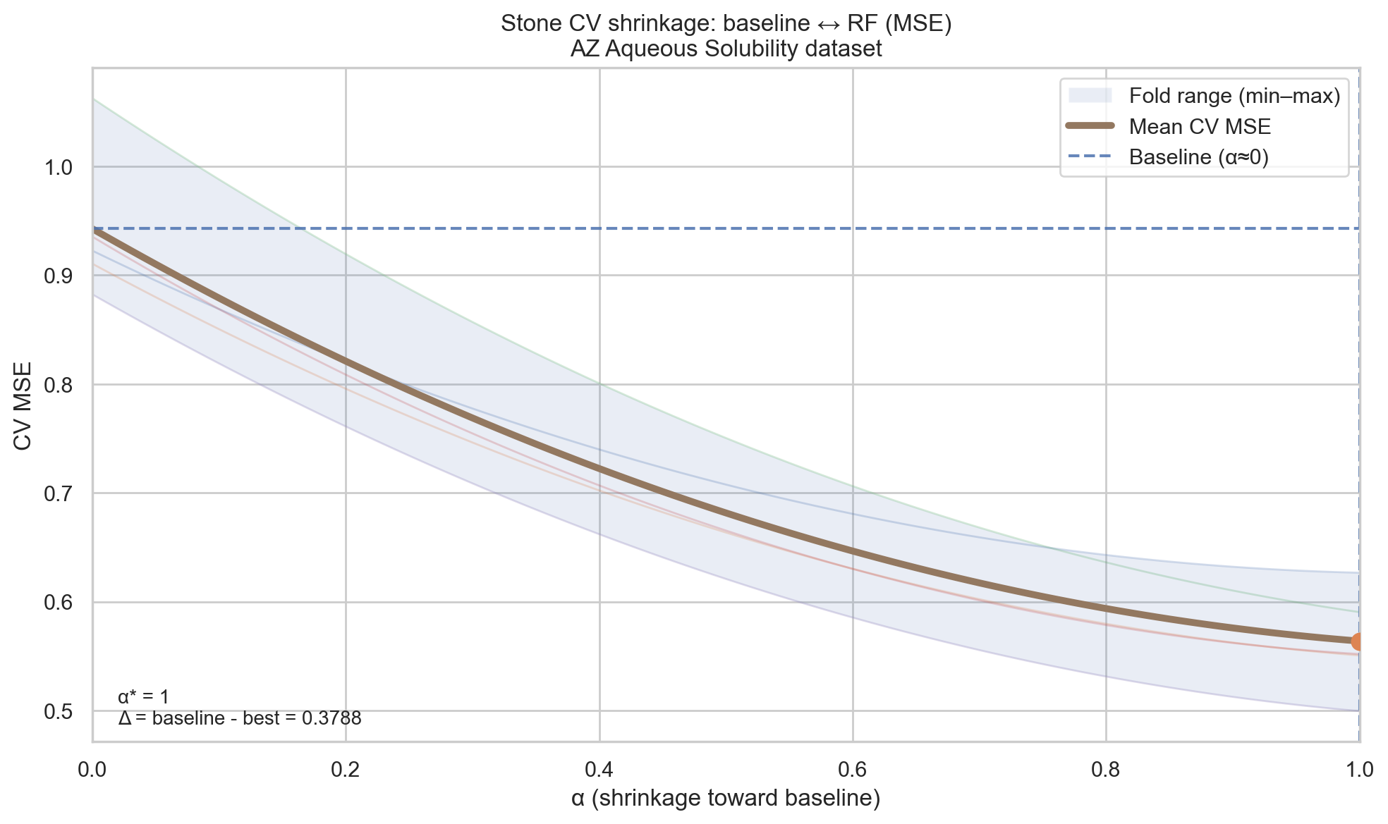
Where \(\bar{y}\) is the most basic estimator of a sample (its mean/average), \(\alpha \in [0,1]\) is a shrinkage factor that gets evaluated during cross-validation.

In each cross-validation iteration, the model gets trained and tested, then the value of \(\alpha\) is changed to take values between 0 and 1. The value that gives the best prediction is the selected value (check Figure 7).

• If \(\alpha = 0\), this eliminates the effect of the model’s prediction and the prediction falls back to the baseline prediction (\(\bar{y}\)).
• If \(\alpha = 1\), this favors the model’s prediction fully.
• If \(0 < \alpha < 1\), this mixes the usage of both the baseline and the model because neither was enough on its own.

So, in Stone’s framework, it was possible to say: None of the models improve over a baseline.

Or, let’s mix the results of these two models by this factor \(\alpha\) to get a better performance.

However, in the current framework, a researcher is forced to pick one of the models regardless of consideration to a baseline (unless the researcher willingly added a baseline model to the comparison).

Restoring Stone’s CV spirit

The current CV framework did not diverge that much from what Stone envisioned. It only got morphed from a shrinkage factor forcibly embedded in the equation to comparing evaluation metrics against each other.

If one wishes to keep using the current framework as it is, there are two ways to make it as Stone envisioned:

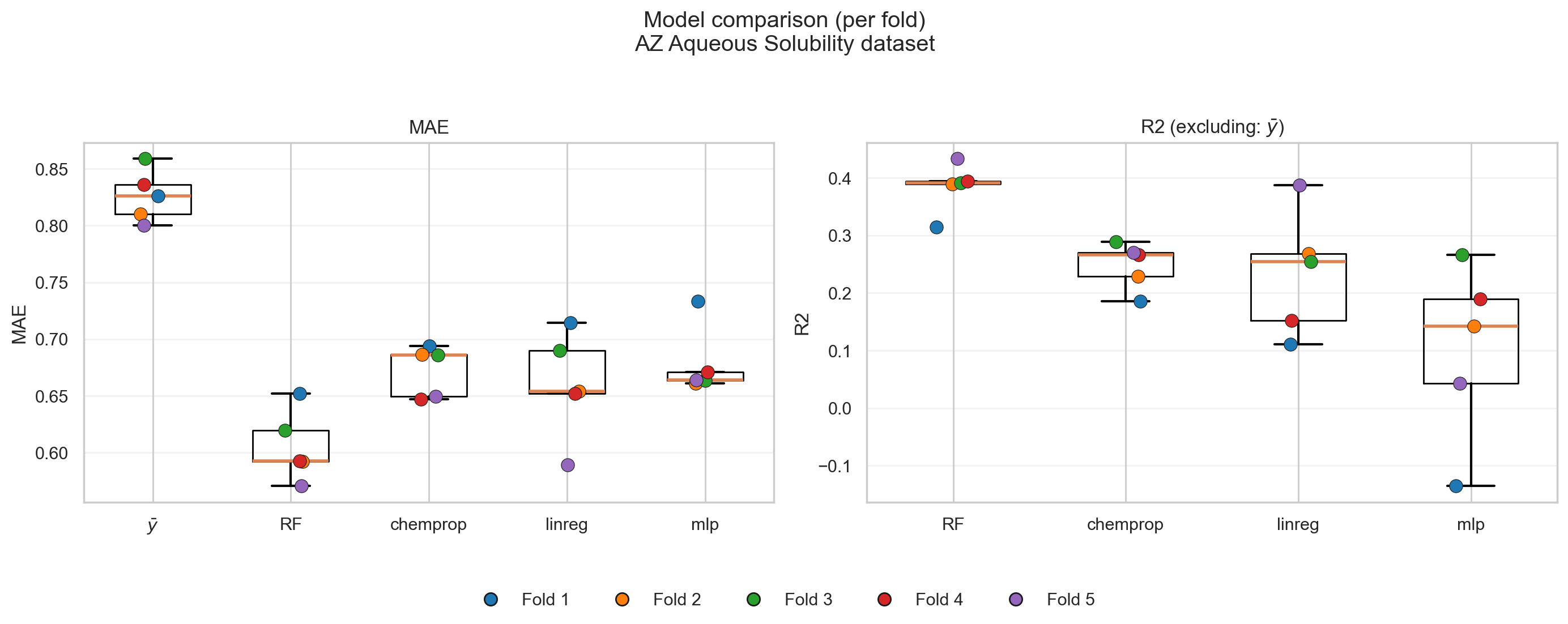
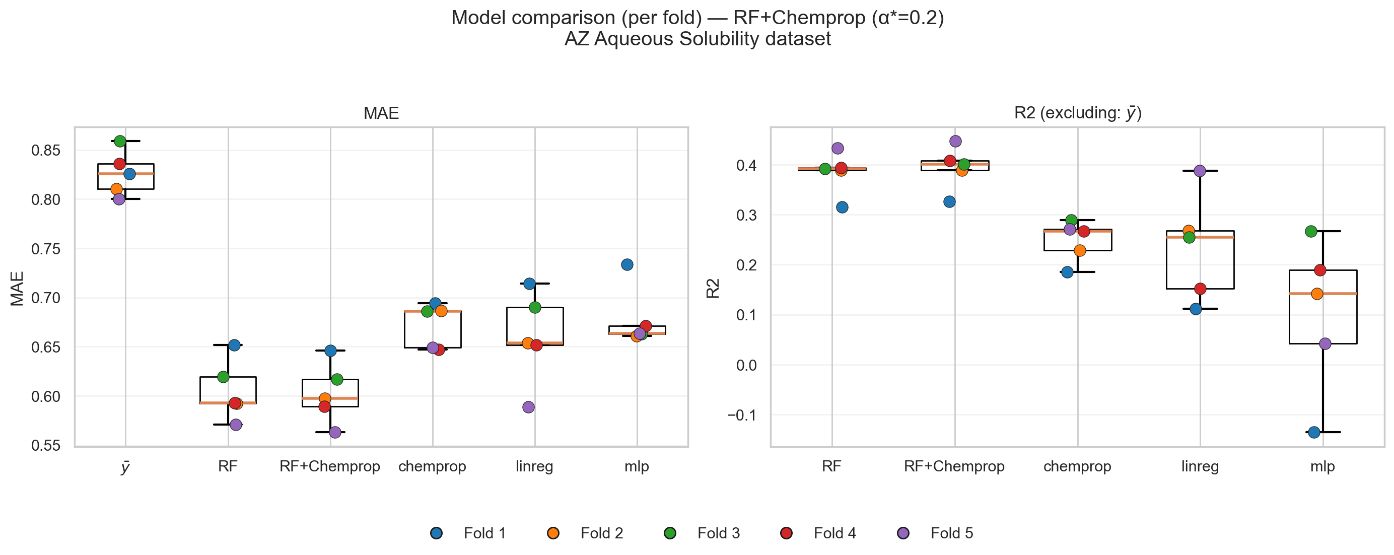
1. Include a baseline model in the comparison of the metric one is using (Figure 8, left).
2. Use a metric that intrinsically compares to a baseline (e.g., \(R^2\)) (Figure 8, right).

The keyword in these two ways is baseline. And this is not a trivially defined word!

Each distribution has a different way to define what is a good baseline. Stone has explained this in his work by showing that his equation would end up approximating the best baseline for different distributions if the model was not the best at capturing the overall structure.

For example, the mean (\(\bar{y}\)) is a good baseline for a normal distribution. However, the median is better for a heavy-tail distribution like cauchy.

To carry this analogy functionally to my field, there are many datasets that would favor the (\(\bar{y}\)) as a statistical baseline. However, there is already evidence that models like random forest (RF) with the RDKit descriptors show up as persistently better models than that baseline (example in Figure 7).

If a researcher develops a complicated method and compares it to (\(\bar{y}\)), they can conclude that their model is superior. However, if RF + RDKit descriptors were a simpler model, then the baseline should change to it rather than (\(\bar{y}\))!

So, when one wants to compare new models to a baseline, it takes time to identify what is a good baseline for the data.

Once this baseline is defined, the conversation shifts to the ways to apply this baseline.

If one is using an evaluation metric like MAE or MSE, it helps to remember that these metrics are mere functions in the actual datapoint \(y_i\) and the prediction by the model \(\hat{y}_i\).

And because these equations are a simple running sum, they are not bounded or standardized. So, they are not intrinsically evaluated against a baseline.

Therefore, the only way to compare such metrics to a baseline is to include the MAE or MSE of this baseline model as one of the viable models to select from (Figure 8, left).

If one uses a metric like \(R^2\), then this metric is intrinsically compared to a baseline. The equation goes like this.

The fraction terms are the MSE equation as shown above. The numerator is the MSE of the model’s prediction, while the denominator is the MSE of the \(\bar{y}\).

If one wishes to rewrite this formula in a more linguistic format, it would be like this:

So, in this equation, a baseline is predefined as the \(\bar{y}\) and the model’s MSE is divided by it. This division term yields a fraction that can range between \([0, \infty]\) (assuming the denominator is never 0).

• If the model’s error is too large compared to the baseline error, the division can theoretically blow up to \(\infty\)
• If the model’s error is too small compared to the baseline, the division can diminish to 0.

Since the final equation is subtracting one from whatever this division results in, the possible range of \(R^2\) is \([-\infty, 1]\), where 1 results when the model’s error is infinitely smaller than the baseline’s error.

Check the below GIF to visualize how MAE, MSE and \(R^2\) are calculated.

Visualization of different regression metrics. MAE sums the absolute difference between true and predicted values without additional considerations. MSE penalizes the error with the square function: a big error gets amplified, and a small error gets rewarded. R2 is normalizing the MSE of the model by the MSE of the baseline mean predictor. This removes the common errors between the model and the baseline, and the fraction that remains describes which model is predicting more accurately.

So, \(R^2\) is already a metric that normalizes the error by a baseline, and the resulting value can tell by how much this model is better than a baseline.

Therefore, if one uses \(R^2\) for comparing their models, they are already halfway in restoring Stone’s spirit.

Why halfway?

Because the denominator term in \(R^2\) forces the usage of \(\bar{y}\) as the baseline. However, as stated earlier, this is not necessarily the best baseline to compare against.

One way to make \(R^2\) fully stone-spirited would be to adapt the equation to have the denominator corresponding to the baseline one would find more suitable (Figure 9).

The missing piece of Stone’s CV spirit

Even though I attempted to understand what exactly Stone meant by his work, and how to align current practices with his vision, there is still one missing piece.

Stone did not propose his CV to “select a model,” but to integrate it to a baseline!

By looking back at the equation Stone presented with his \(\alpha\) factor:

He was not asking: Is the new model better than the baseline.

He was asking: How much can this model improve my baseline.

The equation assumes that \(\bar{y}\) is already encapsulating information, and the other term with \(\alpha\) multiplied by the model’s prediction is possibly providing additional information.

That’s why he was summing the two terms together.

Because both terms can end up mattering together.

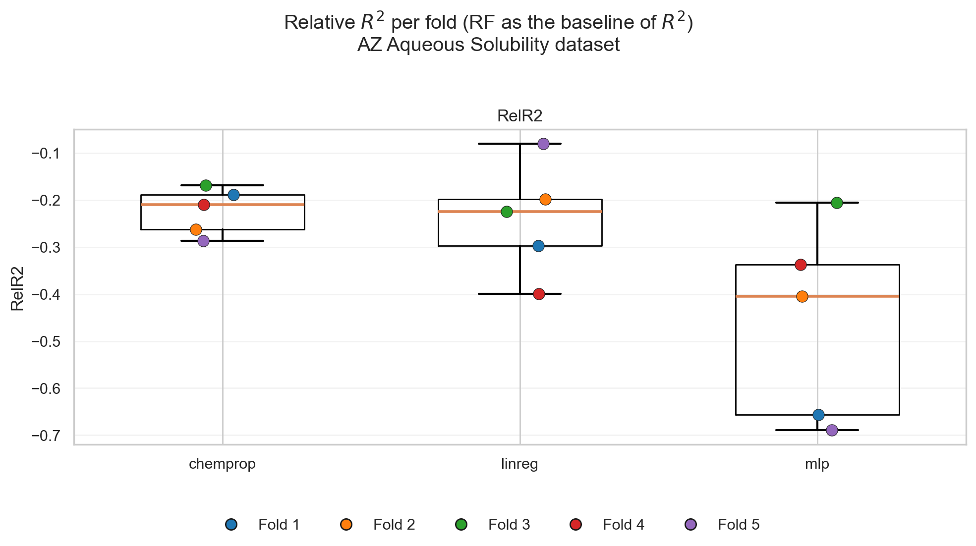
Figures 10 and 11 show how Stone’s CV would have been used to compare models and select a “best runner.” In these figures, RF + RDKit is considered a baseline, Chemprop is considered a promising model, and the \(\alpha\) factor guides one to whether to integrate both models or pick one of them (Figure 10).

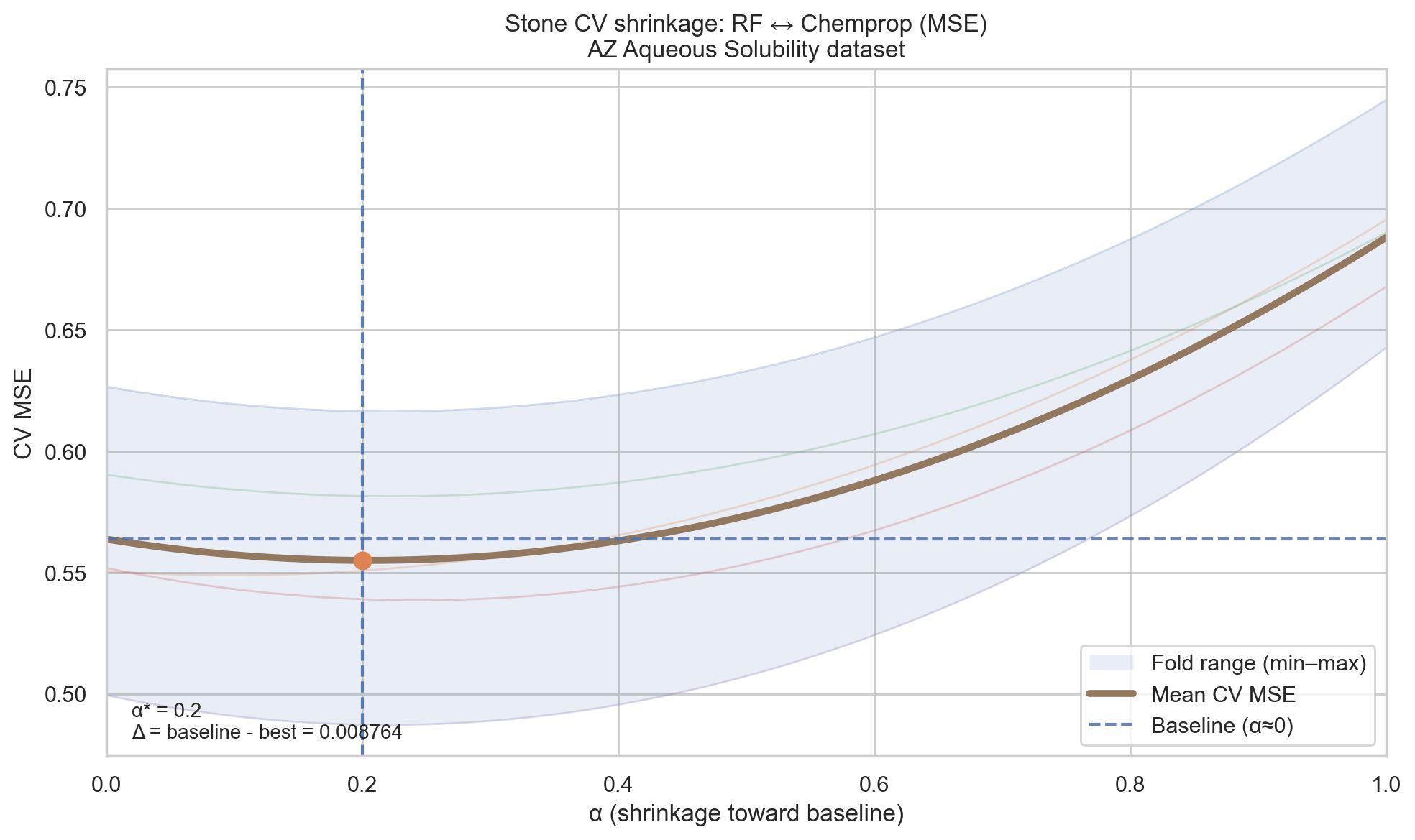
Figure 11 then shows the performance of this new combined model compared to the other models.

Stone’s missing piece from current ML practices is to stay rooted in the last best-working version!

To build models that improve alongside what is already here, rather than “just building models”!

If one wants to incorporate this piece of Stone’s work, it is hard to escape the reality that practices need to change accordingly…

Why stone’s CV (and its restored spirit) still not enough?

Stone’s CV tries to pick a function that would—alongside a stable baseline—prove useful for predicting the underlying data.

His framework is concerned with the premise that the uncertainty lies primarily in the choice of predictor, not in the meaning or validity of the data itself.

Therefore, an honest adherence to Stone’s work would be to make sure that the only variable in the experiment one runs is the choice of the predictor (i.e., the model).

Current k-fold CV splits the data into folds that can be large (e.g., a single fold is 353 datapoints in my example). And due to complications that will be discussed shortly, one can end up with folds that look significantly different from each other.

This ends up with two variables changing during the experiment: the choice of the predictor, and the underlying data itself.

If CV favors the performance of one model over another, the source of this superiority matters:

• Is it because the model’s rationale is solid?
• Is it because the data is heterogeneous?
• Is it both?

Each question can lead the analysis and judgment of the model into a whole different route…

Now, after reading Stone’s paper, I believe the guy was super-intelligent and visionary. In 1974, he thought of many examples that cover stable machine learning practices right now in 2026!

I would like to believe that such a potential hiccup would have caught his attention.

And he did!! Not by mentioning it explicitly, but by emphasizing the importance of domain knowledge.

In his paper, he wrote the following:

“… it is reasonable to enquire how one arrives at a prescription (model) in any particular problem. A tentative answer is that, like a doctor with his patient, the statistician with his client must write his prescription only after careful consideration of the reasonable choices, suggested a priori by the nature of the problem or even by current statistical treatment of the problem type. Just as the doctor should be prepared for side-effects, so the statistician should monitor and check the execution of the prescription for any unexpected complications.”

Stone made an indispensable condition for his framework to succeed: speaking to an expert of the problem and working together to solve it.

Unfortunately, in today’s working atmosphere, problems got complicated, and communication got isolated…

Me, and every cheminformatician who is working in isolation from the people who produce the data, are too oblivious to be selecting a model for this data!

Picking a model requires understanding the data, understanding my representations, and understanding the side effects of my choices, as Stone wrote.

If my data was coming from a psychological or social experiment, for example, it would have been easy for me to understand features like “age” or “marital status” that would be describing my data.

But data from chemistry and drug discovery couldn’t be further from intuitive.

One of the features each researcher in our field uses when deploying RDKit descriptors is called BCUT2D_CHGHI.

What is this feature? What does it mean? What is its typical range? When should I be concerned about its behavior?

I have no idea. These are not trivial questions that I can answer by wandering in my brain.

I will need to consult the original source that proposed it, understand the function that generates it, understand its possible edge behavior, etc.

And this is just a single feature of possible other 210 features provided by RDKit. Another platform like Mordred offers over 1800 features.

The challenge is not just in the features used, but also in the intrinsic process of data generation!

Chemists generate data by tools they understand, with hypotheses they form, with limitations they are aware of, with nuances known to them, etc.

Even if I understood the features, I can still fall short on understanding how the data was generated, and this can lead me into curating—or working with—a chemically faulty dataset.

I have stumbled upon such an example of a dataset that fell short of chemical knowledge when it was curated (check the example mentioned at the end of this post)

So, why is Stone’s CV approach on its own still not enough for today’s challenges?

Because it is concerned solely with the choice of predictor, with an assumption that people communicate together when they are not the expert of the problem.

But… the reality is… cheminformaticians, and every interdisciplinary professional, are not experts at all the intersecting fields they are working with.

We are a mere bridge. A communication tool.

We make people from different areas understand each other because, while they know nothing about each other’s field, we know things from all of them.

And we can make the communication happen…

If communication with experts is missing, an interdisciplinary professional ends up either:

1. Failing to produce something that works.
2. Being forced to be the expert in all the fields themselves…

Final remark

I was worried that I would be putting my own words in Stone’s mouth.

I feel largely aligned with what I understood from his paper. But there is always this risk that one is reading what “they believe” in someone else’s text rather than what the person “actually wrote.”

Until I read this paragraph written by Rex Galbraith in the obituary for Stone.

“… Much of this work involved reading and comprehending voluminous (and often badly explained) technical reports, which he did with no remuneration and little support, motivated only by a desire (to) improve society and to expose nonsense. He was particularly scathing about the misuse of statistics in NHS funding formulae and the unwarranted claims made about them. At the end of a paper that he was working on when he died, he wrote of himself:
“One of Mervyn’s few concessions to everyday social grace was the straight face he tried to keep about econometrics’ thoughtless use of additive linear modelling of the real world in its glorious diversity”…”

Now, I can be a bit relieved that, even if I put words into Stone’s mouth, they won’t feel that foreign from what he himself would have said!

Let’s recap

• Cross-validation felt intuitive for model comparison, but this intuition started to look misleading in practice without careful considerations.
• “Model comparison” here means comparing performance distributions on truly unseen (ideally i.i.d.) data.
• If a single test set is large and representative, different CV folds should not add new information… only confirm the same distribution.
• If folds behave differently, the alarm can be about data heterogeneity / violated assumptions, not about “which model wins.”
• Stone’s 1974 CV frames evaluation around improving a baseline (and possibly integrating models), but modern workflows often ignore baseline + domain-knowledge constraints