In my first blog post, I made two bold statements about transformer models for molecular property prediction in our review¹ — namely, that they fall short in terms of both novelty and benchmarking. In this and the following posts, I hope to convince you of these conclusions.

I’ll walk you through my not-so-easy, still-in-progress journey to answer the question:

Once I’ve finished training my ML model, how good will it perform on new data?

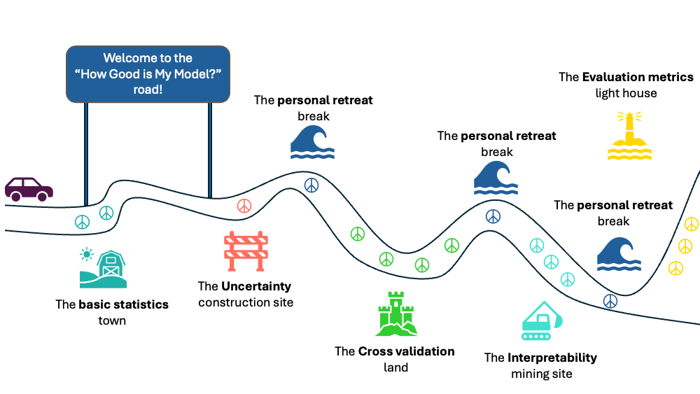
The answer will be a series of blog posts spanning different topics that — in my opinion — all need to be tackled together to be able to answer these questions. In the below sketch, I outline a rough terrain of what this journey will look like, but the journey is still being in progress, and detours can happen along the road as needed.

This post in the series begins with points that may seem extremely trivial to those who’ve been doing machine learning for years. However, I highly recommend being patient and listening to a kid who has something to say — and is very enthusiastic about it! Seeing the world through a kid’s eyes can sometimes be refreshing.
Worst-case scenario: if one encounters a student struggling with a seemingly simple concept, this might offer a new intuitive way to help them out.

This post is also accompanied by a notebook to reproduce the figures and explore the concepts shown below.

TL;DR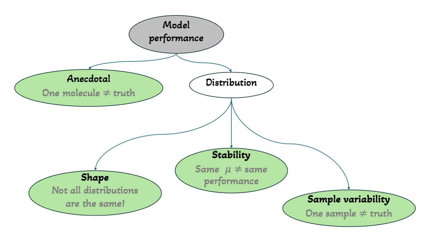

Motivation

Ever since I started working on our review¹, I’ve kept asking myself:

• But, what does an RMSE of 0.5 mean? Does it matter if it’s 0.5 or 0.52?
• Why are different metrics being reported? What does each one really mean?
• If my model is 0.05 better than another — is that enough to claim superiority?

For the first year and a half of my PhD, these were the questions that kept me up at night and were my core motives when working on our recent manuscript that is now available on arXiv.
A lot of effort went into making the manuscript trustworthy, and I’ll now lay out the thought process that went, and still going, to answer these questions.

It’s not a new or groundbreaking answer — just connecting dots that have been floating in the collective knowledge space for decades.

Setting the Stage

Let’s start by describing the playground in which I’ll be unpacking these concepts in the next blog posts.

I imagined training an ML model to predict the aqueous solubility of a molecule. Aqueous solubility measures how much of a molecule can dissolve in water before saturation. Take salt, for example, it dissolves easily — but keep adding more, and eventually, it stops dissolving and begins to settle at the bottom. This point of ‘no more dissolving’ is the aqueous solubility moment.

Oversimplifying a bit, solubility is an equilibrium: breaking a compound’s intermolecular bonds, and forming new ones with water. If a compound breaks apart easily and its fragments are comfortably binding to water, it tends to be more soluble — and vice versa.

Solubility is typically expressed in mol/L, indicating how many moles of a substance can dissolve in a liter of water. In the pharmaceutical domain, the more common unit is LogS, the base-10 logarithm of mol/L².

Now, imagine I have access to the LogS values for millions of diverse molecules. The goal of predictive ML is to take these vast, diverse molecules and find patterns that explain why one has a solubility of -0.5 LogS and another has -4 LogS.
With access to a huge dataset, one often assumes that all the learnable patterns are already embedded in the data — and that it’s just a matter of choosing the right representation and algorithm to extract them.

In that case, I could just throw all the ML models I know at the problem and then jump to the evaluation metrics part of this series to evaluate these models’ performance and make my pick.

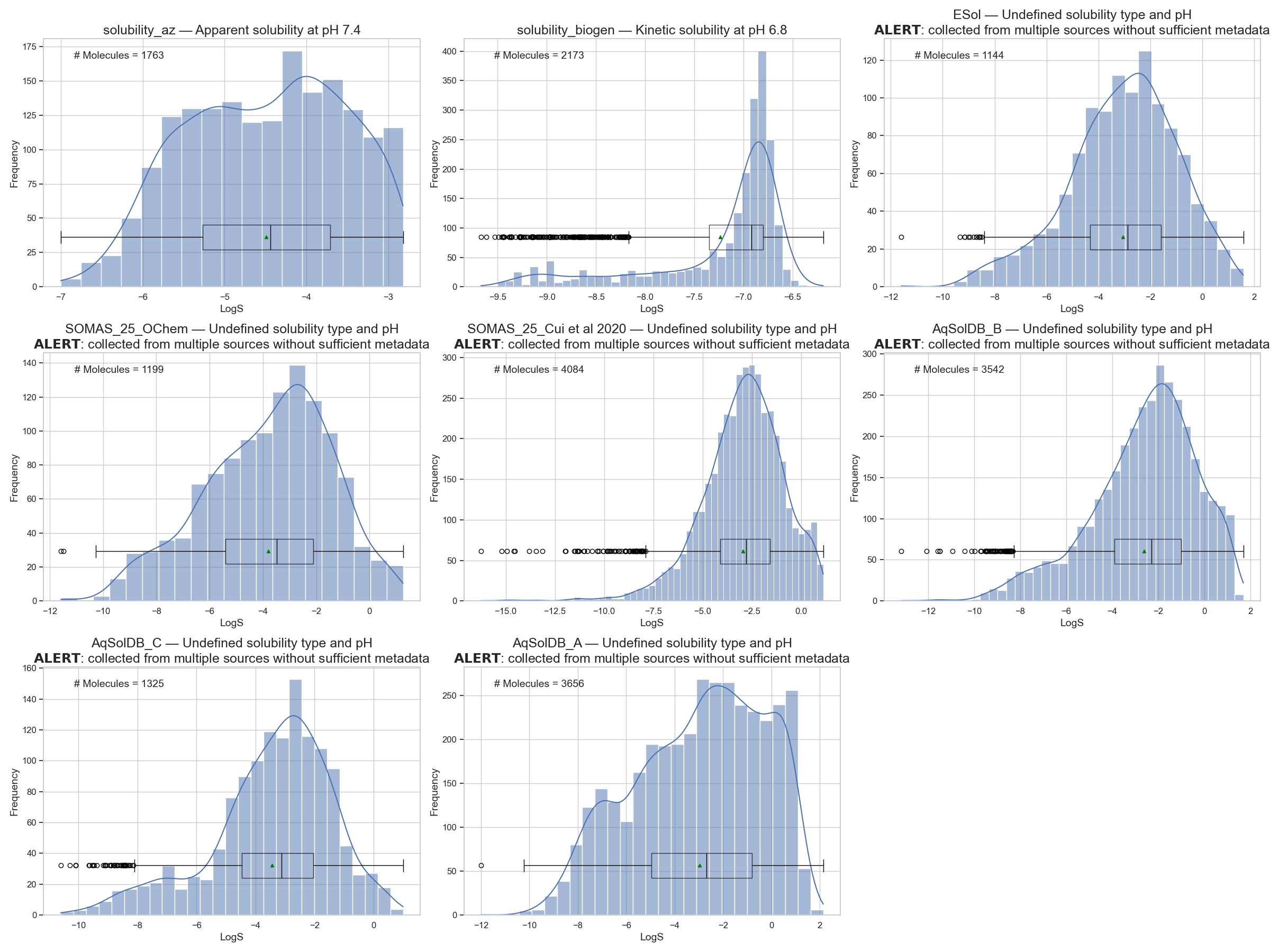
But in reality, we usually have access to small datasets — just a few thousand molecules (Figure 2). That’s why I’ll need to unpack the process of evaluating my model through multiple blog posts before attempting to jump to the final answer.

So, when I’m limited to just a few thousand molecules, the simplest thing I can do is choose an algorithm, feed it these molecules, let it work its magic — and wait.

One day, my chemist asks me to predict the solubility of a new molecule. The model says -2 LogS. The chemist tests it — it turns out to be -2.05 LogS. My model was only 0.05 LogS off³.
Not bad at all, right?

But wait — does that mean my model will always be 0.05 LogS off?

What if next time, my model predicts -3.7 LogS, but the actual value is -5.8 LogS? Yikes. That’s way off. Should I throw away the model?

Both cases are anecdotal. They don’t tell us much. To properly say “my model’s error is x LogS”, one needs to report the expected error value.

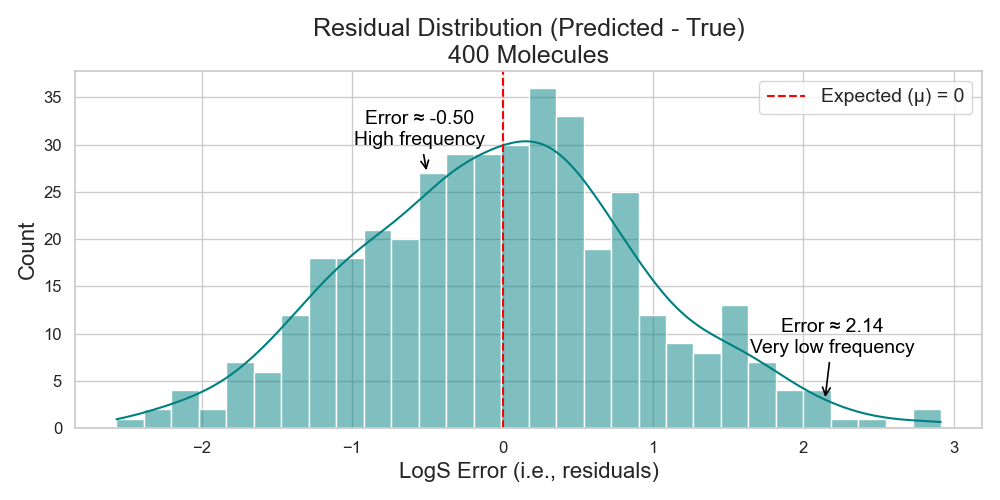
To do that, one must test their model on enough new molecules, plot the distribution of the error for each molecule, and find this expected value (Figure 3).

Takeaway:

One can’t judge a model based on anecdotal errors — distributions matter.

But… what is “the expected value”?

In statistics, the expected value is the mean/average (µ) of a distribution.

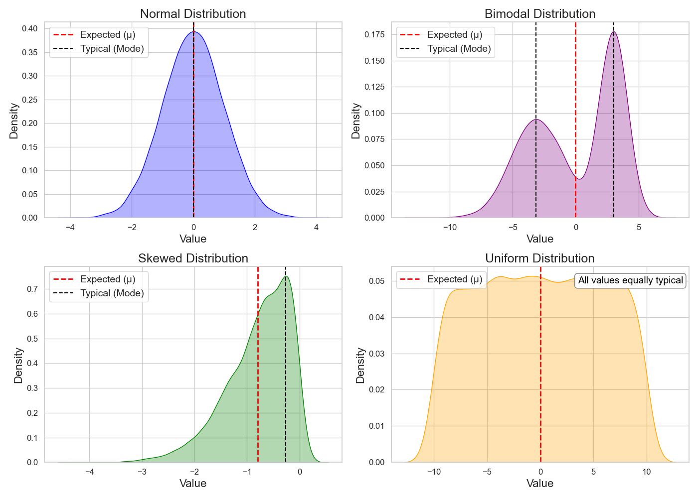
However, when I got into the habit of inspecting my model’s performance distributions, I noticed that for many such distributions, the expected value is not always the most probable value (i.e., typical, where most errors cluster)!

So when everyone was reporting their model’s average performance, I thought that this must be the best representative value. But…

If I report an expected error of 0.05 LogS, but in reality, 60% of my model’s errors are closer to 1 LogS (i.e., the distribution is skewed) — have I really represented my model’s performance honestly?

The expected (mean) and typical (mode) differ depending on the shape of the distribution. This equivalence — expected value equals typical value — holds only for a normal distribution (Figure 4)!

The tradition of reporting mean error comes from an ideal assumption in ML — that the model’s expected error follows a normal distribution, or that approximating this mean will follow one⁴.

But in reality — which is most of the time — that’s not the case.

Once I noticed this, I stopped trusting single numbers. I started looking at distributions.

So, let’s talk in distributions!

Now that I’ve differentiated expected vs. typical, I’ll continue using expected error to describe my model’s error — because it’s the standard in the literature, and much of the subsequent analysis depends on it — but I’ll always remind myself of the nuance behind the term.

So after testing on enough new molecules and identifying the expected error, a transparent statement would be:

“My model’s expected error is x LogS after being tested on n new molecules.”

But realistically, I can’t wait for my chemist to test n new molecules every time.
So, ML folks came up with a clever workaround: train–test split.

We split the available data into two parts:

• A large portion for training,
• A smaller, held-out portion for testing — simulating how the model might perform on real-world, unseen data.

For example, with 2K molecules, I might use an 80:20 split:
→ 1600 for training, 400 for testing.
Those 400 are now my surrogate chemist queries — and they must be treated as unseen.

So now, after testing my model on these 400 new molecules and calculating the expected value, can I say my model’s expected error is x LogS and start comparing it to the expected error of other models?

Not quite.

Standard Deviation: How Stable Is My Model?

The expected error tells us the average case — but what about how much the errors vary around that average?

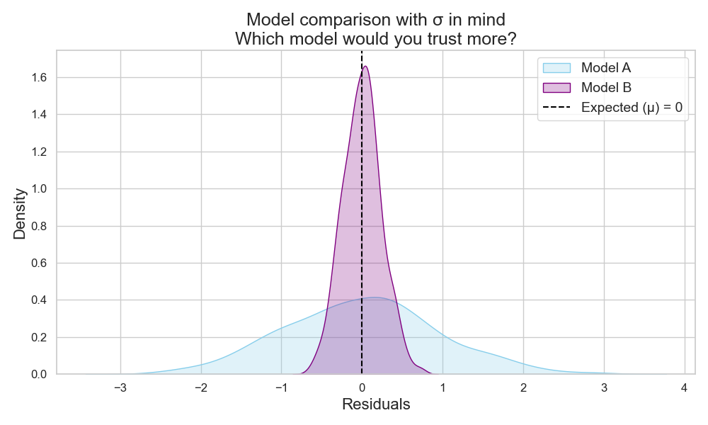
This is where standard deviation (σ) comes in.

σ measures the average distance between each error and the mean (µ).

• A large σ means errors are spread out (less consistent).
• A small σ means errors are clustered tightly around the expected value (more consistent).

⚠️ This intuition holds best for normal distributions — one needs to always check their distribution!

So, if two models have the same expected error, the one with lower σ is more stable and more trustworthy (Figure 5).

Takeaway:

One would need to report both expected error (µ) and standard deviation (σ) of a test set distribution.
When models perform similarly on average, σ helps select the more consistent one.

So is that it? Is testing on a few hundred new molecules and reporting µ and σ all one needs?

Nope…

Beware of sample variability!

Even if I know my model’s µ and σ on these few hundred molecules, can I be confident that testing the model on a new couple of hundred molecules will give the same expected error?

Likely not.

Small sample sizes (like 400 or 200) introduce sampling variability. Sometimes those samples resemble training data, sometimes they’re very different. The model’s performance can fluctuate with each new sample of molecules.

In Figure 6, I show a simulation of the error distribution for a test set containing 10K molecules — I’ll call it the Gold Standard. In the same plot, I show the error on 2000 molecules of this Gold Standard distribution, however, I divided it into 10 small samples, each of size 200 molecules.

As one can see, even tho the small samples are coming from the Gold Standarddistribution, none of the samples’ expected errors captured the true expected error of the Gold Standard distribution. And this is the main problem with small test sets. A single one is not enough to showcase the full performance possibility of a model.

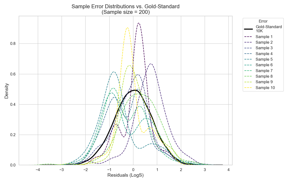
So, unless I have a large and representative hold-out test set, I cannot say with confidence whether the expected error obtained from a single small test set reflects the true expected error of my model.

With this, I come full takeaway circle:

Reporting expected error from a small test set is not enough to estimate my model’s true expected error — just like a single prediction wasn’t enough to estimate the expected error of my model.

Wrapping Up

Let’s summarize:

• One needs to test their model on enough new molecules to estimate a model’s expected error (µ).
• The expected error may differ from the typical error depending on the distribution shape.
• Standard deviation (σ) tells us how stable the model is.
  • If two models have close expected errors, the one with lower σ is more reliable.
• A large, representative test set gives the most trustworthy performance.
  • A small test set provides only an estimate — subject to the quirks of the included data.

But…

What if I don’t have access to a large test set (which is usually the case in our field)?
Is all hope lost?

Fortunately, statistical techniques exist that help estimate these values even with small datasets — more on that in the next post!